Does the weights setting affects the performance of the two-factor portfolio?
Table of Contents
The common weights settings are equal-weighted and capitalization-weighted. The former treats all factors as the same, assigns equal weights to different factors, and synthesizes new factor values; the latter weights individual factors with capitalization-weighted to synthesize new factor values at first, assign different factors with equal weights, and then synthesize new factor values. However, neither of the two methods considers the effectiveness of the factors.
The article considers the effectiveness of factors by adding the IC-weighted, IC describes the correlation between factor value and the subsequent rolling stock returns. If IC value is high, it means the factor is more effective at the moment. When we adjusts dynamically weights at the beginning of each month, factors with higher IC value has higher weights.
Windows OS and Jupyter Notebook
#Basic function and Visualization
import pandas as pd
from scipy import stats
from collections import OrderedDict
import matplotlib.pyplot as plt
import copy#TEJ
import tejapi
tejapi.ApiConfig.api_key = 'Your Key'
tejapi.ApiConfig.ignoretz = True
Step 1. Obtain the stock price, ROE and financial statements date
# 撈取上市所有普通股證券代碼
code = tejapi.get("TWN/EWNPRCSTD", paginate=True, chinese_column_name=True)
code = code["證券碼"][(code["證券種類名稱"] == "普通股") & (code["上市別"].isin(["TSE"]))].to_list()# 匯入 ROE變數
data_ROE = tejapi.get('TWN/AIFIN',
                      coid = code,
                      mdate= {'gte': '2019-01-01','lte':'2020-12-31'},
                      opts={'pivot':True ,'columns':['coid', 'mdate', 'R103']},
                      chinese_column_name=True,
                      paginate=True)# 匯入 財報發布日
data_annouce = tejapi.get('TWN/AIFINA',
                          coid = code,
                          mdate= {'gte': '2019-01-01','lte':'2020-12-31'},
                          opts={'columns':['coid', 'mdate', 'a0003']},
                          chinese_column_name=True,
                          paginate=True)# 匯入 調整後開盤價、收盤價與股價淨值比
data_PB_price = tejapi.get('TWN/APRCD1',
                           coid = code,
                           mdate= {'gte': '2019-03-01','lte':'2020-03-31'},
                           opts={'columns':['coid', 'mdate','open_adj','close_adj','pbr_tej']},
                           chinese_column_name=True,
                           paginate=True)
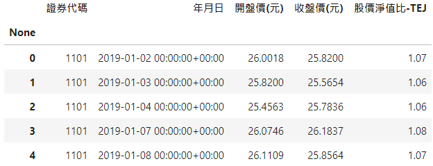
First obtain all listed company codes, and use TEJ API to obtain the financial information in different databases at once.
Step 2. Data Preprocessing
# 整理股價
data_PB_price = data_PB_price.rename({'證券代碼': '公司'}, axis=1) # 改名字
data_PB_price['開盤價(元) t+1'] = data_PB_price.groupby('公司')['開盤價(元)'].shift(-1)# 新增年與月
data_PB_price['年'] = data_PB_price['年月日'].dt.year
data_PB_price['月'] = data_PB_price['年月日'].dt.month
data_PB_price = data_PB_price.sort_values(by=['年月日']).reset_index(drop=True) # 排序年月日
Step 3. Merge data in different frequencies and keep each month end data
# 合併季頻率 ROE與財報發布日
data_all = pd.merge(data_ROE ,data_annouce ,how = 'left' , on = ['公司','年/月'])
data_all = data_all.rename({'年/月': '財報'}, axis=1) # 改名字
data_all = data_all.sort_values(by=['財報發布日']).reset_index(drop=True) # 排序財報發布日# 合併季頻率與日頻率資料
data_all = pd.merge_asof(data_PB_price ,data_all ,left_on = '年月日', right_on = '財報發布日', by = ['公司'] ,direction = "backward")# 留下每月底資料
data_all = data_all.drop_duplicates(subset=['公司','年','月'], keep='last')
data_all = data_all.sort_values(by=['公司','年月日']).reset_index(drop=True)
data_all['月持有報酬率'] = data_all.groupby('公司')['收盤價(元)'].shift(-1).reset_index(drop=True) \
    / data_all['開盤價(元) t+1'] -1
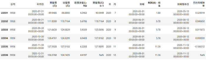
pd.merge and pd.merge_asof are very useful tools to merge dataframes. The former is used to merge data in the same frequency, the latter is used to merge data in the different frequencies. The parameter direction = backward can avoid the look-ahead bias; pd.drop_duplicates can filter the data for year and month, then keep month end data of each company. Finally, we can get the current accurate factor value, and sort and group factor by value.
Step 4. Delete missing data
data_all = data_all.dropna().reset_index(drop=True)
data_all = data_all.set_index(['年月日','公司'])
data_all = data_all[['股價淨值比-TEJ','ROE(A)-稅後','月持有報酬率']]
Step 1. Sort a factor based on value
def get_rank(data):
    factors_name=[i for i in data.columns.tolist() if i not in ['月持有報酬率']] # 得到因子名

    rank_df = []
    for factor in factors_name:
        if factor in ['股價淨值比-TEJ']:
            rank_list = data[factor].groupby(level=0).rank(ascending = True) # rank由小到大排序,即值越小,排名越靠前
        else:
            rank_list = data[factor].groupby(level=0).rank(ascending = False) # rank由大到小排序,即值越大,排名越靠前

        rank_df.append(rank_list)

    rank_df = pd.concat(rank_df, axis=1)
    return rank_df
ROE is a measure of a company’s profitability, a company with a higher ROE has greater the expected rate of return, so it is arranged in descending order, that is, ROE is higher, the ranking is higher; PE ratio is a measure of a company’s good value, a company with a lower PE ratio has greater the expected rate of return, so it is arranged in ascending order, that is, PE ratio is more small, the ranking is higher.
Step 2. Get IC values
def get_ic(data):
    factors_name=[i for i in data.columns.tolist() if i not in ['月持有報酬率']] # 得到因子名
    ic = data.groupby(level=0).\
        apply(lambda data: [stats.spearmanr(data[factor],
                                            data['月持有報酬率'])[1] for factor in factors_name])

    ic = pd.DataFrame(ic.tolist(), index=ic.index, columns=factors_name)
    return ic
IC is a correlation coefficient of the factor to the future holding rate of return at a certain cross-sectional time. The higher IC value, the higher the expected return of holding in the future. IC can be used to compare different effectiveness factors.
Step 3. Synthesize new factor
# 根據IC計算因子權重
def ic_weight(data):
data_= data.copy()
ic = get_ic(data)
ic0 = ic.abs() # 計算 IC絕對值
rolling_ic = ic0.rolling(12,min_periods=1).mean() # 滾動 12个月
weight = rolling_ic.div(rolling_ic.sum(axis=1),axis=0) # 計算 IC權重,按行求和,按列相除
ranks = get_rank(data) # 得到各因子的排序數據
score_ = OrderedDict()
for date in weight.index.tolist():
rank = ranks.loc[date]
score = rank * weight.loc[date]
score_[date] = score.sum(axis=1).to_frame().rename(columns={0: 'score'})
score_df = pd.concat(score_.values(),keys=score_.keys())
score_df = score_df.reset_index().rename({'level_0': '年月日'}, axis=1)
score_df = score_df.set_index(['年月日','公司'])
data_ = data_.join(score_df)
data_ = data_.reset_index()
return data_data_ic = ic_weight(data_all)
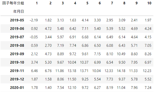
data_ic['因子每年分組'] = data_ic.groupby('年月日')['score'].rank().\
transform(lambda x: pd.qcut(x, 10, labels = range(1,11)))
Step 1. Calculate portfolio’s monthly return
def arrange_group_return(tempt):
    tempt = tempt.groupby(['年月日','因子每年分組'])[['月持有報酬率']].mean().reset_index()
    tempt['月持有報酬率'] = tempt['月持有報酬率'] * 100
    tempt = pd.pivot_table(tempt, values='月持有報酬率', index=['因子每年分組'] ,columns=['年月日'])
    tempt.index = tempt.index.astype(str)
    tempt = tempt.T
    tempt = tempt.cumsum().dropna()
    tempt.index = tempt.index.astype(str).str[:7]

    return temptdata_ic = arrange_group_return(data_ic)data_ic.round(2)
Step 2. Visualize the cumulative rate of return of the grouping
def draw_group_return(tempt ,weight_method):
fig = plt.figure(figsize = (14,7))
ax = fig.add_subplot()
ax.set_title(weight_method,
fontsize=16,
fontweight='bold')
for i in tempt.columns:
ax.plot(tempt[i], linewidth=2, alpha=0.8 , marker='o')
ax.legend(tempt.columns,loc=2)
plt.grid(axis='y')
plt.xlabel('日期', fontsize=18)
plt.ylabel('報酬率 %',rotation=0, fontsize=18,labelpad=20)
plt.xticks(fontsize=12)
plt.yticks(fontsize=12)
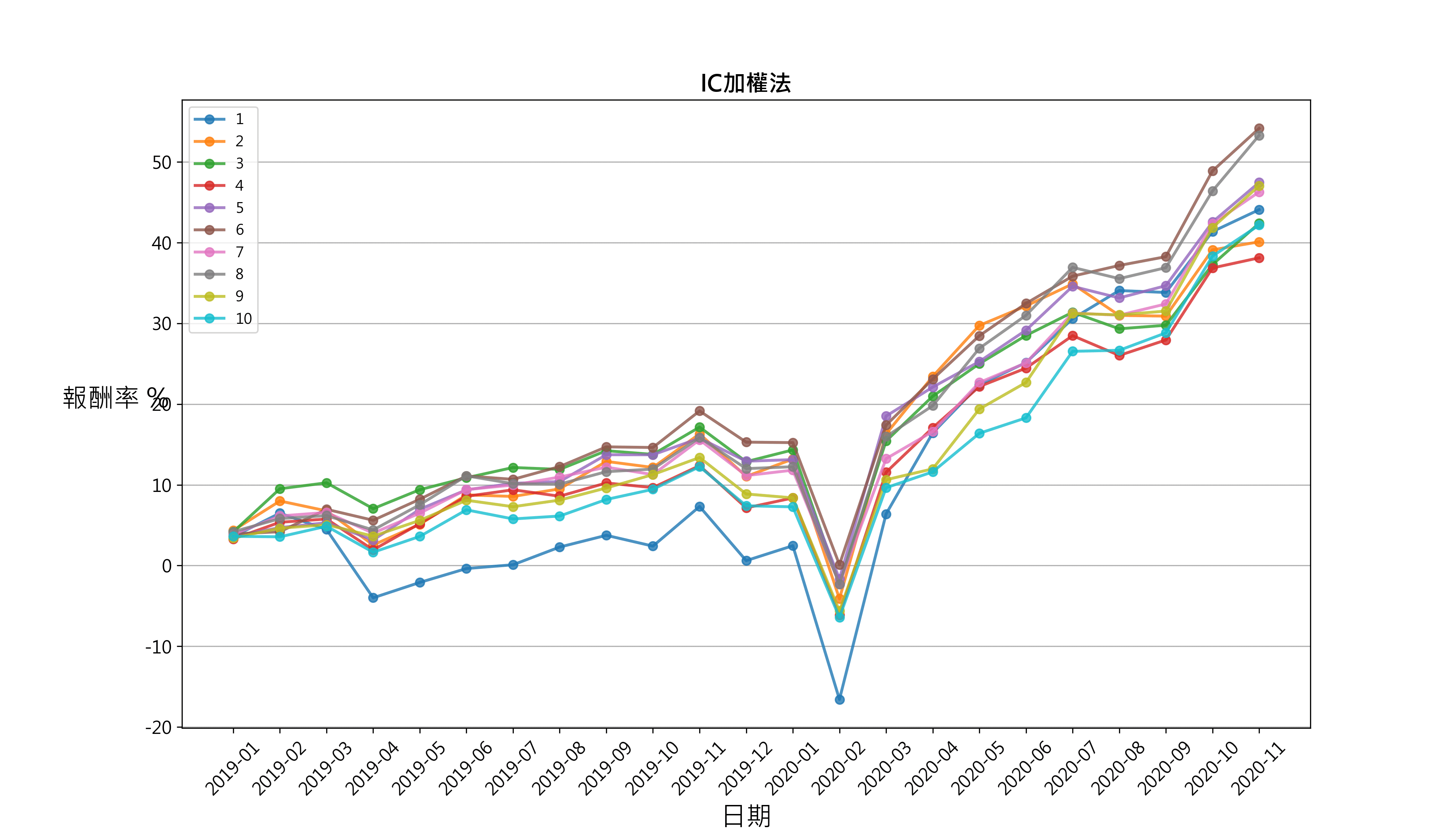
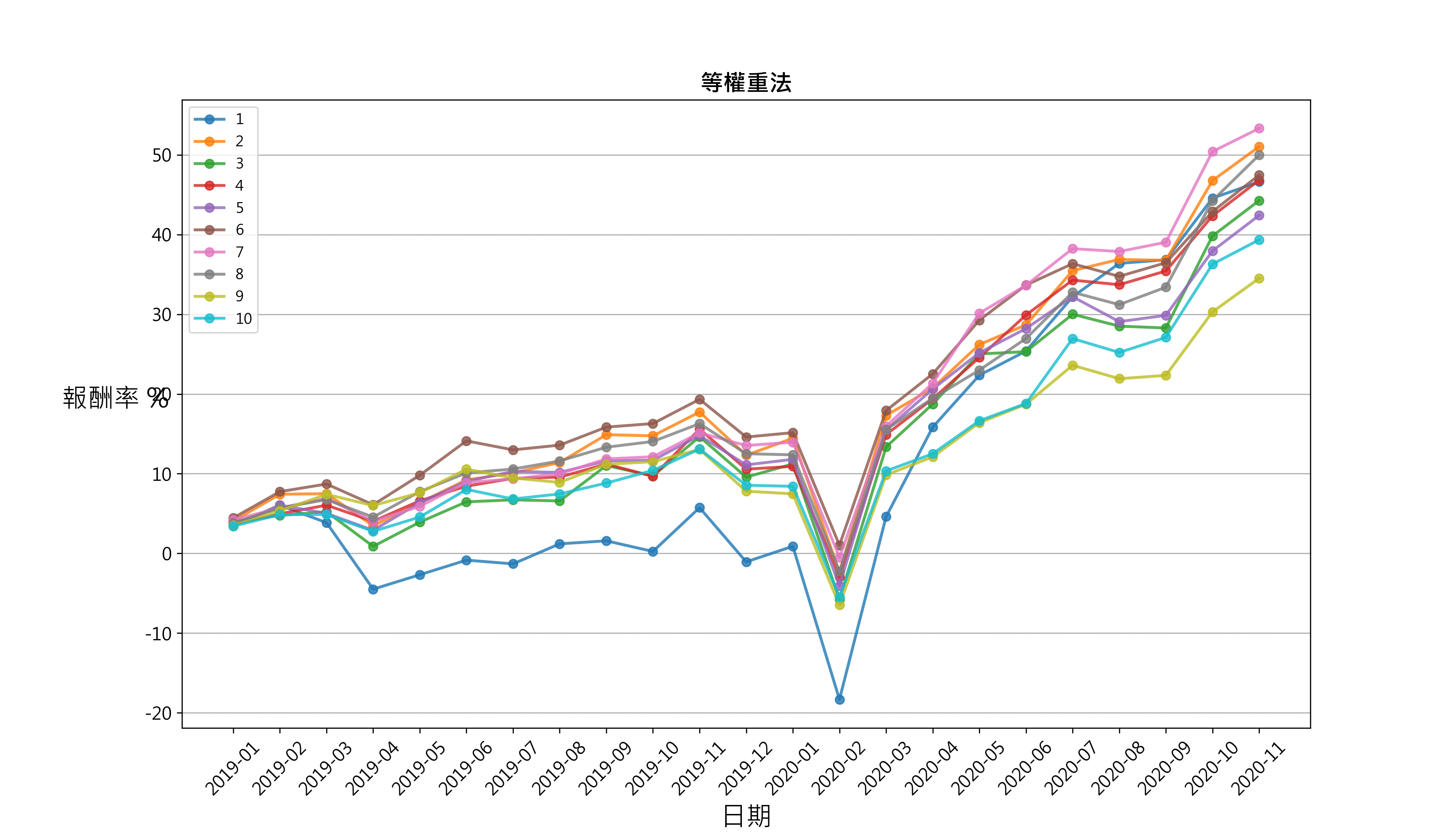
plt.show()draw_group_return(data_ic, 'IC加權法')
# 比較 等權重法與 IC加權法
data_equal_ir = pd.merge(
pd.DataFrame(data_equal['1']).rename({'1':'等權重法'}, axis=1),
pd.DataFrame(data_ic['1']).rename({'1':'IC加權法'}, axis=1),
how='inner',left_index=True, right_index=True)draw_group_return(data_equal_ir, '等權重法 vs IC加權法')
Compare the first group of the two weighting methods, that is, the group with the largest ROE and the smallest PE ratio.
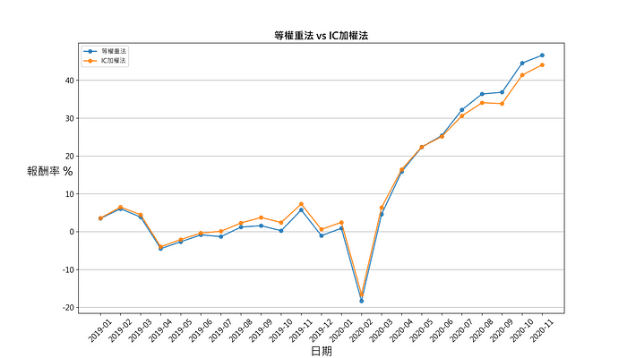
The synthetic factor portfolio performance of PE ratio and ROE does not show a stable monotonicity and discrimination from the beginning of 2019 to the end of 2020. Monthly frequency transaction and quarterly ROE data are the reason why cumulative rate of return of the grouping is sometimes tangled. Meanwhile, The equal-weighted and the IC-weighted have no significant difference in different time periods.
We can try to reduce the frequency of transactions in the future and backtest different factor combinations to find stable monotonicity and discriminative factor combinations, and then further optimize the factor weights. If readers are interested in other factor information, welcome to purchase the plan offered in TEJ E-Shop and find the factors with profitability, stability and interpretability!
