Observe the relation between employee turnover rate and stocks return

Table of Contents
In recent years, there’s an investment called ESG investing, meaning when investing, the firm’s financial performance is not the only thing to be considered. Instead, its influence over environment and society and its corporate governance should be stressed as well. There are no trade-off relations between each other, but a virtuous cycle that promises the future prospect of the firm, bringing tremendous wealth for the investors.
Factor investing is intended to find some key factors that will help earn excessive return. For example, according to the literature, size factor, book to market factor and risk factor are common factors in this regard. Therefore, this week we use “employee turnover rate” provided by TEJ database as our factor, and see how ESG investing works !
Windows OS and Jupyter Notebook
#Basic
import pandas as pd
import numpy as np
import plotly.express as px
import plotly.graph_objects as go
#TEJ
import tejapi
tejapi.ApiConfig.api_key = 'Your Key'
tejapi.ApiConfig.ignoretz = True
turnover = tejapi.get('TWN/ACSR01A',
        paginate = True,
        opts = {'columns':['coid','mdate','turn_rate','num_staff']},
        chinese_column_name = True)
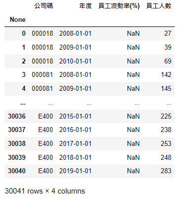
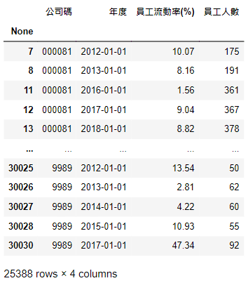
turnover = turnover[turnover['員工流動率(%)'].isnull() == False]
result = pd.DataFrame()
ret_table = pd.DataFrame()
Since the employee turnover rate is disclosed in annual report, to avoid look-ahead bias, we take the deadline of disclosing annual report as our portfolio formation date, which is the end of next year’s March and we will hold the portfolio for one year. However, based on the approach, the portfolio built on 2020 information will be held between 2021–03–31 and 2022–03–31, which currently has no complete one-year-return. Thus, we will exclude this year.
date_list = sorted(turnover['年度'].unique())[:-1]
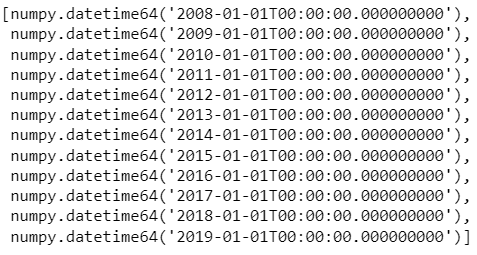
Next, we use loop to calculate the return of each year’s portfolios. We will use the first year (date = ‘2008–01–01’) to demonstrate how each loop works in detail. The complete code can be viewed in source code section
#Choose this year's data
data = turnover[turnover['年度'] == date].reset_index(drop=True)#Remove the firm with few employees
data = data[data['員工人數'] >= data['員工人數'].quantile(0.1)]#Grouping
data['group'] = pd.qcut(data['員工流動率(%)'], q=10,labels = [i for i in range(1,11)])#Store
result = result.append(data)
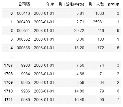
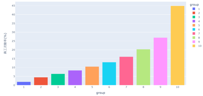
First of all, choose that year’s data and remove the firm with few employees (less than 10th quantile). Then, use the function pd.qcut() to form 10 groups by turnover rate and show the group number in new column group. Finally, store it in result
#Sell date of portfolios
sell_date = date + pd.Timedelta(days = 365 + 90 + 365)

#to store data and portfolio return
port_ret = [date]
2008-based portfolios will be sold in 2020–03–31. The date (2008–01–01) and these 10 portfolios’ return will be stored in list port_ret
#Calculate this year's portfolios' return
for group in range(1,11):

      #this year, certain group
      sub_data = data[data['group'] == group].reset_index(drop=True)

      #Obtain return
      ret = tejapi.get('TWN/APRCD2',
                   coid = sub_data['公司碼'].tolist(),
                   mdate = {'gte':sell_date - pd.Timedelta(days = 5), 'lte':sell_date},
                   opts = {'columns':['coid','mdate', 'roi_y']},
                   paginate = True,
                   chinese_column_name = True)

       #Get the data closest to sell date
       ret = ret.groupby(by='證券代碼').last().reset_index()

       #Portfolio return(%)
       port_ret.append(ret['年報酬率 %'].mean())
#Table
ret_table =  ret_table.append(pd.DataFrame(data = np.array(port_ret).reshape((1,11)), columns = ['日期'] + [i for i in range(1,11)])).reset_index(drop=True)
Next, we use for loop to go through each group. For starters, we choose the group’s data and obtain annual return based on the firms’ codes and sell date. The tip here is we first select the several days’ return before the sell date, and get the return that’s closest to sell date, which is the annual return over the past one year. Lastly, we take average and get equally-weighted return. After calculating all groups’ return, we will store them in list port_ret, transform it to a dataframe and store in ret_table

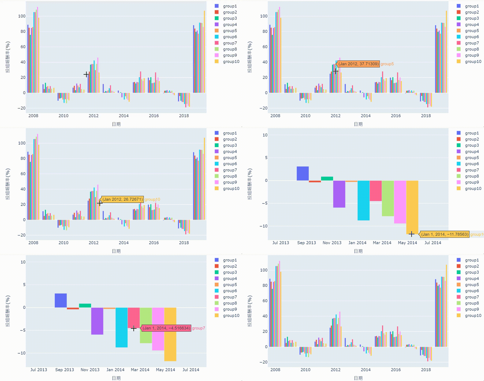
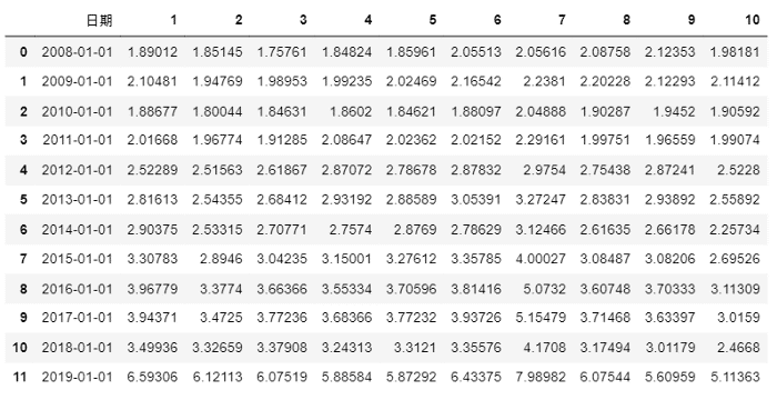
Other years follow the same procedure. Through each loop, result and ret_table are updated as follows

cum_ret = ret_table[[i for i in range(1,11)]].apply(lambda x : (x*0.01 + 1)).cumprod()
cum_ret.insert(0, '日期', date_list)
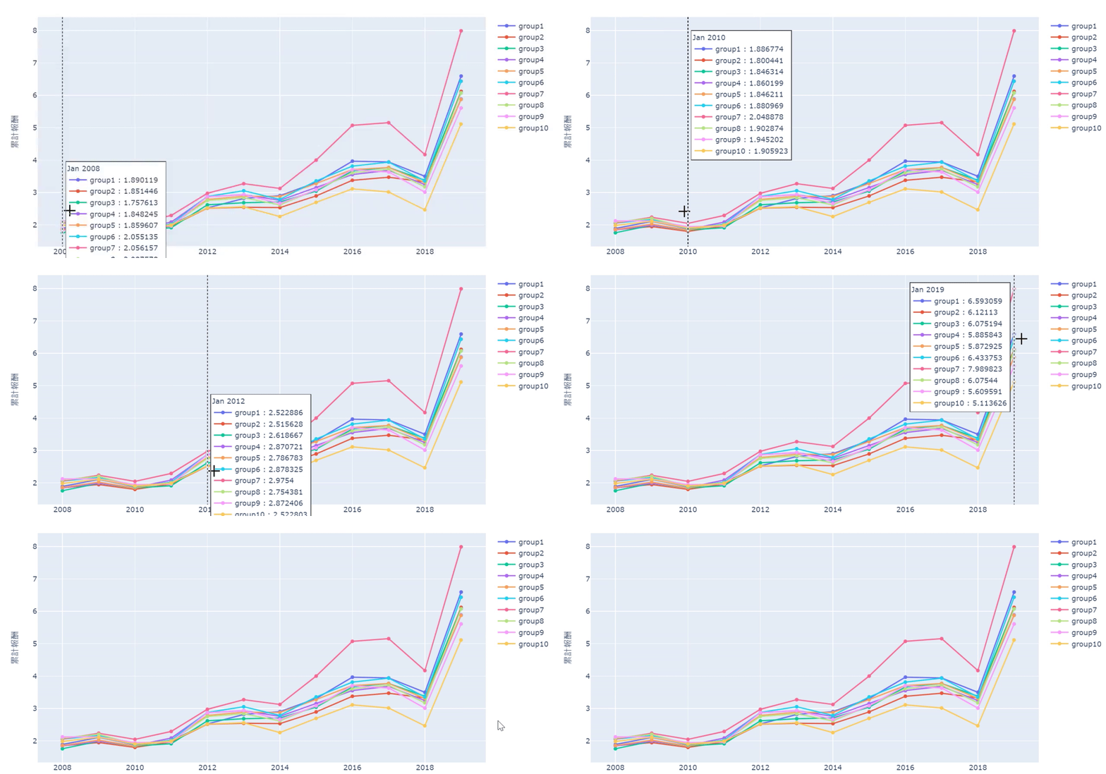
Calculate cumulative return for these ten portfolios and insert the date back
sharpe_list = []
for i in range(1,11):

    #Annual return
    cagr = (cum_ret[i].values[-1]**(1/len(cum_ret)) - 1)*100

    #Annual standard deviation
    std = ret_table[i].std()

    #Update list
    sharpe_list.append(i)
    sharpe_list.append((cagr-1)/std)#Form a table
sharpe = pd.DataFrame(np.array(sharpe_list).reshape((10,2)), columns = ["group","夏普比率(%)"])
Calculate the sharpe ratio first, then visualize it
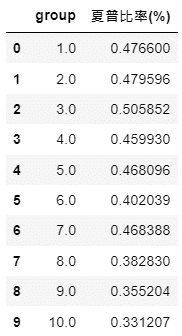
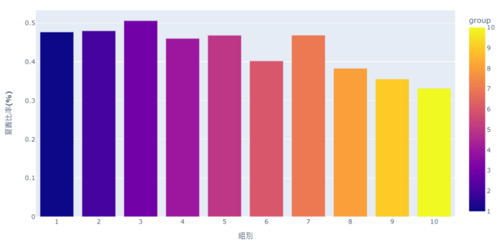
From the cumulative chart and sharpe ratio, it’s shown that the 10th group (the highest turnover rate’s group) has the worst performance, even though it has good performance in certain years. However, it doesn’t necessarily mean the lowest turnover rate is the best. For example, from cumulative chart we know it’s 7th group that is the best instead of the 1st group. Probably, it implies maintaining a certain degree of employee turnover rate can make firms more competitive and energetic
Overall, in the bear market, the firms with higher turnover rate tend to loss more, meaning ESG investing may provide downside risk protection. If readers are interested in other ESG factors, welcome to TEJ E-Shop to choose the optimal plan and find out more profitable factors !