
If you’ve been involved in investing for some time, you’ve likely heard a lot about algorithmic trading and quantitative trading strategies. For beginners with no software or coding background, it might seem daunting at first. However, with the rise of AI in recent years, the ability to automate investment strategies could become an essential tool for future investors. One of the significant advantages of algorithmic trading is its ability to overcome the “weaknesses of human nature effectively”! This article will guide you through a tutorial on algorithmic trading, highlighting the differences between algorithmic and manual trading. We’ll start with the basic algorithmic trading concepts, gradually introduce you to the field, and help you master the skills needed for algorithmic trading!
Table of Contents
Algorithmic trading means using code or automated tools to execute trades when investing. This includes all the typical investment processes, such as researching and identifying relevant stocks, performing fundamental or technical analysis, and executing orders. All these processes are automated through programming, which we call “algorithmic trading.”
Many often hear “algorithmic trading” and “quantitative trading.” What’s the difference between the two? Algorithmic and quantitative trading are essentially the same; both involve using programs to place orders or execute investment strategies to achieve automated investing. The difference is merely in the terminology.
Algorithmic trading not only requires more advanced investment knowledge, but it also has a relatively higher barrier to entry. So why do some investors choose algorithmic trading? The reason lies in its three key advantages, which cannot be replicated by discretionary (manual) trading.
The most significant advantage of algorithmic trading is “automation.” Computers don’t get tired, but people do. With algorithmic trading, you can save significant time by not having to constantly sit in front of your computer to monitor the market. It can perform the same tasks as a human trader, significantly reducing time costs.
Whether you rely on fundamental analysis, market sentiment, or technical analysis, you must look at various “data” such as financial statements, institutional trading activity, or technical indicators. Algorithmic trading allows for real-time monitoring of these data points, enabling you to monitor market conditions 24/7 and never miss any market changes.
Another advantage of algorithmic trading is the ability to perform “backtesting.” Backtesting involves using the same investment strategy to calculate past performance to see if the strategy would have been profitable. With algorithmic trading, you can quickly backtest strategies, using data to assess the strategy’s feasibility objectively.
| Algorithmic Trading | Manual Trading (Discretionary Trading) | |
| Basis for Trades | Trades based solely on pre-set program criteria, following indicators or data. | Trades based on human subjective judgment, which may involve intuition, fear, or greed. |
| Trading Time | 24/7 automated trading | Limited to available free time |
| Trading Tools | Requires software with API integration; not all trading platforms support this. | Any trading software, or orders can be placed through a broker. |

What is a trend? The commonly seen market conditions like “bear markets” or “bull markets” are examples of trends. The trend strategy involves using various technical indicators, such as EMA (Exponential Moving Average), MACD (Moving Average Convergence Divergence), KDJ, or the Williams %R indicator, to determine the direction of the trend and trade “in line” with it. For instance, if the trend is upward, you would go long; if it’s downward, you would go short.
Momentum Strategy:
The momentum strategy involves “weeding out the weak and keeping the strong.” It involves immediately following a stock when it starts to show significant potential and momentum. This is one of the advantages of algorithmic trading (the ability to monitor and place orders to follow momentum quickly). There is also an advanced “dual momentum” strategy. Typical indicators used include the Momentum (MTM) indicator, Average True Range (ATR), and the Relative Strength Index (RSI).
Contrarian Strategy:
The strategies mentioned earlier are essentially trend-following strategies, but many investors also adopt contrarian strategies. A contrarian strategy involves “betting on tops or bottoms,” where you predict that the market is about to reverse and take a position accordingly. Typical indicators this strategy uses include the Bias (BIAS) indicator, the Parabolic SAR, and the Pivot Point analysis.
Capital Flow Strategy:
Capital flow refers to the activities of institutional investors and major players, including foreign investors, investment trusts, proprietary traders, and large investors. The capital flow strategy involves tracking and following the movement of these capital flows. The advantage of algorithmic trading here is its real-time ability to monitor capital movements. When large investors begin buying or selling, the program can place trades accordingly. Typical indicators include the short-interest ratio, extensive shareholder holdings, and institutional buying and selling data.
Fundamental Strategy:
Don’t assume that algorithmic trading must focus solely on technical analysis. Many value investors who emphasize fundamental analysis also choose to implement algorithmic trading. The basic strategy includes financial statement analysis, macroeconomic indicators, and industry metrics, all of which can be considered in algorithmic trading. Common indicators include the cash flow statement, balance sheet, and gross profit margin.
Many people wonder what types of assets are suitable for algorithmic trading. The answer depends on the characteristics of algorithmic trading:
Algorithmic trading is not limited to specific assets. It thrives in markets with large volumes, such as U.S. stocks, cryptocurrencies, and commodities like gold and oil. However, its adaptability is a key strength. Whether used for real-time notifications or data detection, algorithmic trading can be beneficial in any market or with any asset, providing traders and investors with a versatile tool.
After understanding the advantages of algorithmic trading, how do you implement it? Next, we will dive into practical examples and exercises in an algorithmic trading tutorial! This time, we will introduce and demonstrate the four essential functions of the TQuant Lab’s zipline-tej applying the buy-and-hold strategy. In this case, we’ll conduct a buy and sell operation on the first and last days of the backtesting period and calculate the performance.
In recent years, TSMC (2330) has shown a long-term upward trend in its stock price, and with its market capitalization accounting for half of the Taiwanese stock market, it has attracted many investors. This example will introduce the zipline backtesting method using the classic buy-and-hold strategy. This will include an overview of the four fundamental functions for building a zipline trading strategy: initialize, handle_data, analyze, and run_algorithm.
We use the os module and the! zipline ingest command in Zipline to import stock price data into the local environment. The standard syntax is:
| !zipline ingest -b tqant |
Here, -b stands for “bundle,” which is a container for the stock price and volume information, and quant is the bundle name, which the user can customize. Before running the ingest command, you need to use os to set environment variables, allowing Zipline to receive the desired assets and date ranges specified by the user. Generally, the syntax for setting environment variables is as follows:

The initialize function is a crucial part of building a zipline trading strategy. It is called once before the backtesting begins and is primarily used to set up the backtesting environment. Common tasks include configuring slippage or commission fees. The following functions are typically used:
Sets the slippage model. Zipline offers four different slippage calculation methods. For details, please refer to the subsequent tutorial on zipline slippage.
Sets the commission fee model. Zipline provides three different commission calculation methods. For details, please refer to the subsequent tutorial on zipline commission.
A typical implementation looks like this:
| def initialize(context): set_slippage(slippage.FixedSlippage()) set_commission(commission.PerShare(cost=0.00285)) |
In addition, the initialize function contains a parameter called context. The context is a namespace that allows you to store various custom variables, which can then be accessed and modified during each trading day loop. For example, you can set a variable context.day = 0 to keep track of the number of trading days and put another variable context.has_ordered = False to record whether TSMC stock has already been purchased.
| def initialize(context): context.day = 0 context.has_ordered = False set_slippage(slippage.FixedSlippage()) set_commission(commission.PerShare(cost=0.00285)) |

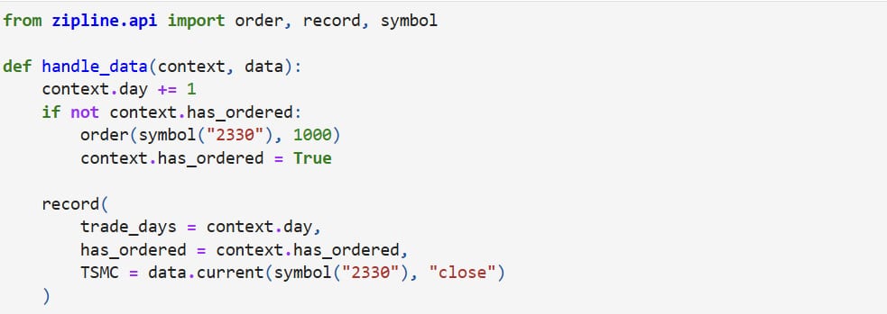
The handle_data function is crucial to building a zipline trading strategy. It is called every day during the backtesting period. Its main tasks are to set the trading strategy, place orders, and record trade information.
The handle_data function contains two parameters: context and data. The context parameter functions the same way described in the initialize section above. To keep track of the trading days and whether TSMC stock is held, we set it up as follows:
def handle_data(context, data):
context.day += 1 # Increment the trading day count.
if not context.has_ordered: # Check if TSMC stock is held. Note that we set the context.has_ordered to False in initialize.
Next, we introduce the order placement function. There are six different types of order functions, which are documented under zipline order-related functions. Here, we use the most basic order function:
zipline.api.order
This function is used to buy or sell a certain number of shares of a given asset.
Parameters:
We then add the order function order(symbol(“2330”)), where symbol(“2330”) is the Asset data type in zipline. After placing the order, we changed context.has_ordered to True, so the order will not be placed again on the next trading day. The updated code looks like this:
| def handle_data(context, data): context.day += 1 if not context.has_ordered: # Order 1000 shares of TSMC (symbol “2330”) order(symbol(“2330”), 1000) # Set context.has_ordered to True to avoid placing the order again on the next trading day context.has_ordered = True |
Finally, we use the record function to record the number of trading days, whether a position is held, and the price of the day. The purpose of this function is to log information for each trading day and include the recorded data in a column format in the final output table generated by run_algorithm. The code for this is written as follows:
| record( 欄位名稱 = 資訊) |
The line (data.current(symbol(“2330”), “close”)) references the data parameter mentioned earlier in handle_data. The data parameter’s main function is to store daily price and volume data and make it accessible for retrieval. In this example, we want to record the closing price of the day, so we use the data.current() function.
zipline.data.current
This function retrieves the price and volume information for a given stock on a specific day.
Parameters:
Since we want to record TSMC’s closing price for the day, the code is written as follows:
| def handle_data(context, data): context.day += 1 if not context.has_ordered: order(symbol(“2330”, 1000) context.has_ordered = True record( # 紀錄用 trade_days = context.day, has_ordered = context.has_ordered, TSMC = data.current(symbol(“2330”), “close”) ) |
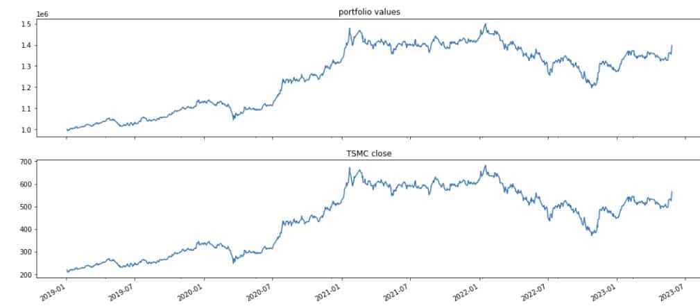
The analyze function primarily visualizes strategy performance and risk after backtesting. We use matplotlib to plot the portfolio value and TSMC’s stock price trends. The analyze function takes two parameters: context and perf. The context parameter functions the same way described above, while perf is the final output table from run_algorithm—also known as results. We can extract specific columns from it to create the charts.
zipline.run_algorithm
Executes the strategy backtest.
Parameters:
start: pd.Timestamp or datetime The start date of the backtest.end: pd.Timestamp or datetime The end date of the backtest.initialize: callable Calls the initialize function for the backtest.capital_base: int The initial capital amount.handle_data: callable, optional Calls the handle_data function for the backtest.before_trading_start: callable, optional Calls the before_trading_start function for the backtest.analyze: callable, optional Calls the analyze function for the backtest.data_frequency: {"daily", "minute"}, optional Sets the trading frequency.bundle: str, optional Sets the bundle to use for the backtest.trading_calendar: TradingCalendar, optional Sets the trading calendar.benchmark_returns: pd.Series, optional Sets the benchmark return rate.treasury_returns: pd.Series, optional Sets the risk-free rate.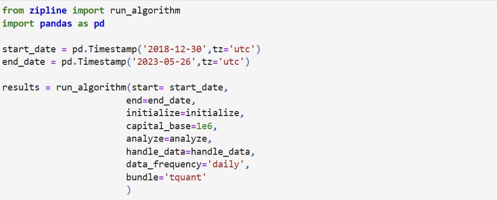
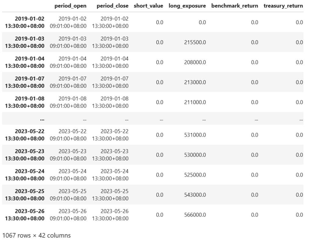
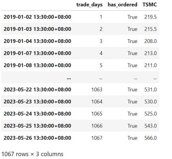
We can observe that the previously used order records for trade_days, has_ordered, and TSMC are indeed recorded as columns in the results table.
results[['trade_days','has_ordered','TSMC']]
When engaging in algorithmic trading, choosing the right platform and tools and considering the market and assets is essential. This is key to maximizing the performance of your algorithmic trading. An ideal trading platform should offer a high-efficiency and stable trading environment, along with precise backtesting capabilities. These capabilities allow for greater flexibility in trading strategies, ensuring that you are ready to adapt to any market conditions and optimize your strategies with ease.
Why is backtesting so important? The reason is that trading strategies are often formulated based on past performance data, making the accuracy of backtesting a crucial indicator of a strategy’s stability. A high-quality backtesting engine should be able to simulate a natural trading environment, considering factors like slippage, transaction fees, and other trading costs. This ensures the results are reliable, helping traders optimize their strategies effectively.
For example, many of the backtesting platforms or suites available on the market today may need more comprehensive backtesting systems. For instance, they may need to offer detailed transaction fees and slippage settings, leading to inaccurate backtesting results and potentially causing investors to make erroneous trades. Additionally, overly simplistic platforms may leave investors without sufficient information to determine if their strategies contain errors or bugs. On the other hand, the TQuant Lab backtesting system offers precise settings for transaction fees and slippage and allows for parameter adjustments to avoid specific events, enabling strategy adjustments, such as setting limits for price fluctuations or stock dividend distributions.
TEJ uses the Zipline toolkit provided by Quantopian, modifying it to align with the Taiwanese financial market’s trading environment and creating a backtesting engine. Over years of development, this backtesting engine has become a foundational structure commonly used in international quantitative platforms. Maintained by TEJ’s professional quantitative analysis team, it is regularly updated with new features, enabling it to backtest various assets, including stocks and ETFs. During the backtesting process, logs automatically display multiple records of the portfolio’s daily stock holdings, including cash dividends, stock dividends, and other information, closely reflecting actual market conditions.
TEJ’s system, built on Quantopian’s Pipeline toolkit, offers a flexible approach to constructing investment factors. It filters and retrieves specific financial data, allowing users to design unique investment strategies. The system automatically shifts data by one period to prevent look-ahead bias. It includes built-in calculation functions such as z-score, SimpleMovingAverage, person, and BollingerBands, making it easier to create customized investment indicators. The system also generates visual process flowcharts, empowering users to understand the strategy calculation process.
The TEJ team has adapted the Alphalens factor analysis tool to the Taiwanese financial market, offering a comprehensive range of factor research and analysis capabilities. The return analysis function allows users to build long-short hedging portfolios to test factor effectiveness quickly. In contrast, the information analysis function can observe whether a factor can predict future stock returns. Moreover, the turnover analysis function can examine the turnover rate of a factor, assessing whether it leads to excessive trading costs. This comprehensive analysis ensures a thorough understanding of the factors at play in the market.
Pyfolio is a powerful strategy performance analysis tool that enables users to quickly grasp a strategy’s strengths and weaknesses. With just one click, you can generate a complete set of performance metrics and produce various visual reports. This tool can analyze a strategy’s performance during major historical financial events to check its robustness. Additionally, Pyfolio can analyze the portfolio’s illiquid stocks, helping identify potential liquidity risks.
Zipline-tej’s event-driven backtesting can simulate market entry and exit conditions, offering various dynamic and static slippage models, such as fixed-point and volume-driven dynamic slippage costs. It also includes Taiwan-specific transaction cost models and order execution delay mechanisms. Combined with trading day annotations provided by the TEJ database, it prevents look-ahead bias in backtests, ensuring that results are more realistic and reliable, such as successfully avoiding the ability to buy during price limits.
Start Building Portfolios That Outperform the Market!