Table of Contents
STREAMLIT、Data Visualization、Grid Trading
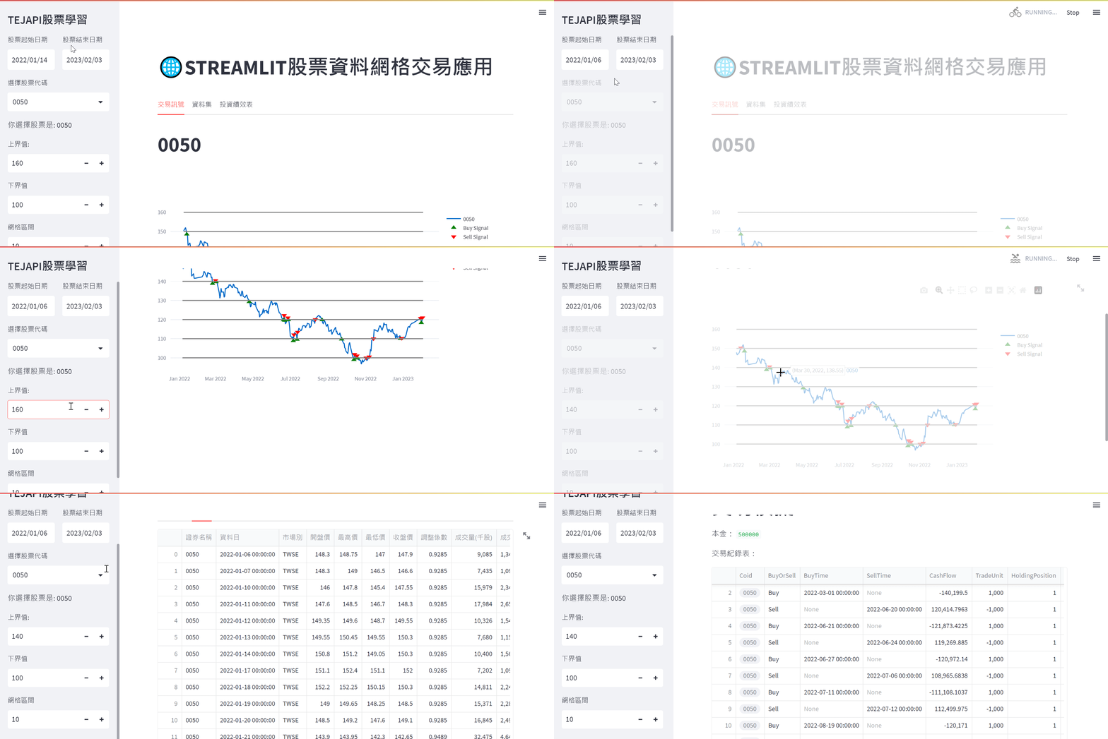
In previous tutorials, we learned how to create our own STREAMLIT App. For more details, you can refer to this article. In this article, we will use the TEJ API database to connect with the STREAMLIT package and implement a grid trading strategy. We will use tools such as date selection, dropdown menus, and numerical selectors to interact with charts and tables, making the data an interactive app.
Grid trading is a trading strategy that selects a range by setting two parameters, the upper bound and the lower bound. We divide the stock price into grid intervals, buying stocks when the price falls and touches the lower grid, and selling stocks when the price rises and exceeds the upper grid.
This strategy is a lazy strategy that doesn’t require much manual operation. It can also profit from price fluctuations. However, there are a few points to note which is the efficiency of capital utilization will be lower than manual trading.

We use Windows and VScode as the editor in this article.
# STREAMLIT套件
import streamlit as st
import pandas as pd
# 可以互動的PLOT套件
import plotly.graph_objects as go
# 設置日期格式的套件
import datetime
from datetime import datetime as dt
from datetime import timedelta
import tejapi

# 登入TEJ API
tejapi.ApiConfig.api_key = your_key
#把時間取消保留日期 (無視)
tejapi.ApiConfig.ignoretz = TrueSidebar Widget Settings

col1, col2 = st.columns(2)
with col1:
        # 將股票起使日期設置為變數d1
        d1 = st.date_input(
        "股票起始日期",
        # 並將預設資料設定為2022年的1/1
        datetime.date(2022, 1, 1))

    with col2:
        # 將股票起使日期設置為變數d2
        d2= st.date_input(
        "股票結束日期",
datetime.date(2023, 2, 3))Since the stock data for the current day has not closed, fetching data for the current day would result in an error. Therefore, we fetch data for yesterday and only keep the “coid” (stock name) column in the “opts” variable.
#輸入股價
# 使用date套件的date獲取今天的日期資料
current_date = dt.now().date()
    # 使用date套件的timedelta獲取昨天的日期資料
    previous_date = current_date - timedelta(days=1)
    data = tejapi.get('TWN/APIPRCD',
                  mdate=previous_date,
                  opts={'columns':['coid']},
                  paginate=True)

    coids = data['coid'].tolist()
    stock_code = st.selectbox('選擇股票代碼', data)
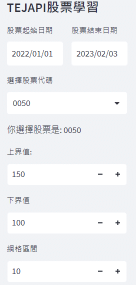
st.write('你選擇股票是: ', stock_code)這邊將預設的值設定為上界值為150、下界值為100、網格區間設定為
upper_bound = st.number_input('上界值:',value=150)
lower_bound = st.number_input('下界值:',value=100)
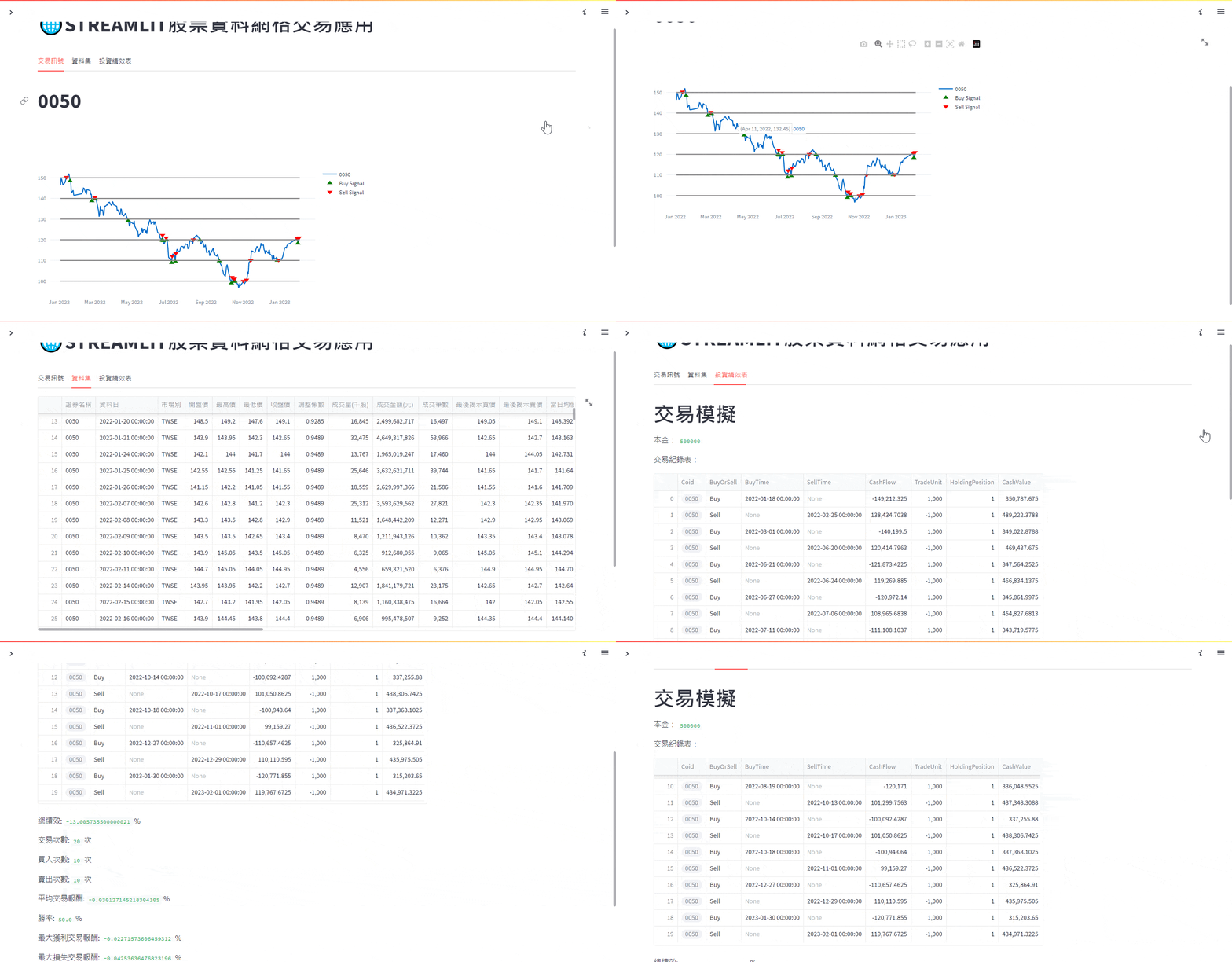
interval = st.number_input('網格區間:',value=10)On the right side panel, we configure three tools to help us observe data trends, including buy and sell signal charts, datasets, and returns.

We have the stock name, start time, and end time on the left side. Here, we input these parameters into our TEJAPI database to select the data we need.
Next, we create fields for buy and sell signals, filling the buy signal with data when the price falls and touches the grid and filling the sell signal with data when the price rises beyond the grid.
stock_id = {stock_code}
    gte, lte = {d1}, {d2}
    tejdata= tejapi.get('TWN/APIPRCD',
                        paginate = True,
                        coid = stock_id,
                        mdate = {'gte':gte, 'lte':lte},
                        chinese_column_name=True
                        )
    df = tejdata
    df.reset_index(drop=True, inplace=True)

    # 創建 Buy_Signal 和 Sell_Signal 列,預設為 False
    df['Buy_Signal'] = False
    df['Sell_Signal'] = False

    # 在適當的條件下,將 Buy_Signal 和 Sell_Signal 設置為 True
    grid = list(range(lower_bound, upper_bound + interval, interval))
    for i in range(1, len(df)):
        for price in grid:
            if df['收盤價'][i-1] > price >= df['收盤價'][i]:
                df.at[i, 'Buy_Signal'] = True
            if df['收盤價'][i-1] < price <= df['收盤價'][i]:
df.at[i, 'Sell_Signal'] = Truetab1, tab2, tab3 = st.tabs(["交易訊號", "資料集", "投資績效表"])將收盤價繪製成股票走勢圖並寫進tab1當中,再將買賣訊號加入在圖表當中
with tab1:
    st.title(stock_code)
    fig = go.Figure()
    fig.add_trace(go.Scatter(x=df['資料日'], y=df['收盤價'], name=stock_code))

    # 創建網格,將線條顏色設置為灰色
    for price in grid:
        fig.add_shape(type="line", x0=df['資料日'].iloc[0], x1=df['資料日'].iloc[-1], y0=price, y1=price, line=dict(color='gray'))

    # 加入買進訊號的散點圖
    buy_signals = df[df['Buy_Signal']]
    fig.add_trace(go.Scatter(x=buy_signals['資料日'], y=buy_signals['收盤價'], mode='markers', name='Buy Signal', marker=dict(color='green', size=10, symbol='triangle-up')))

    # 加入賣出訊號的散點圖
    sell_signals = df[df['Sell_Signal']]
    fig.add_trace(go.Scatter(x=sell_signals['資料日'], y=sell_signals['收盤價'], mode='markers', name='Sell Signal', marker=dict(color='red', size=10, symbol='triangle-down')))
    fig.update_layout()
st.plotly_chart(fig)Input the data retrieved earlier into “tab2” and add a data download button.
with tab2:
    st.dataframe(df, height=500)
    @st.cache_data
    def convert_df(df):
        # IMPORTANT: Cache the conversion to prevent computation on every rerun
        return df.to_csv().encode("utf-8")
    csv = convert_df(df)

    st.download_button(
        label="點此下載資料範例",
        data=csv,
        file_name=f"{stock_code}股價資料.csv",
        mime="text/csv",)
- principal: Initial investment
- position: Number of shares held in the position
- cash : Amount of cash held
- order_unit : Number of shares traded in each transaction
Here, we set the principle to 500,000 and the number of shares bought or sold in each transaction (order_unit) to 1000 shares. We will create a new dataset called trade_book to record transaction time, transaction cost, trading units, holding positions, and cash value. We will use the parameters in this dataset to calculate investment performance.
The column names in the trade_book transaction table are as follows:
- BuyTime: Buy time
- SellTime: Sell time
- CashFlow: Cash inflow/outflow
- TradeUnit: Number of shares bought/sold
- HoldingPosition: Current position
- CashValue: Remaining cash amount
with tab3:
    st.title('交易模擬')

    # 初始化本金和交易紀錄表
    principal = 500000
    cash = principal
    position = 0
    order_unit = 1000  # 每次交易的股數
    trade_book = pd.DataFrame(columns=['Coid', 'BuyOrSell', 'BuyTime', 'SellTime', 'CashFlow', 'TradeUnit', 'HoldingPosition', 'CashValue'])

    st.write("本金:", principal)

    # 進行網格交易並更新交易紀錄表
    for i in range(1, len(df)):
        cu_time = df['資料日'][i]
        cu_close = df['收盤價'][i]
        n_time = df['資料日'][i - 1]
        n_open = df['開盤價'][i]

        if position == 0 and df['Buy_Signal'][i]:
            # 判斷是否進行買進
            position += 1
            order_time = n_time
            order_price = n_open
            friction_cost = (20 if order_price * order_unit * 0.001425 < 20 else order_price * order_unit * 0.001425)
            total_cost = -1 * order_price * order_unit - friction_cost
            cash += total_cost
            trade_book = trade_book.append({'Coid': stock_id, 'BuyOrSell': 'Buy', 'BuyTime': order_time, 'SellTime': None, 'CashFlow': total_cost, 'TradeUnit': order_unit, 'HoldingPosition': position, 'CashValue': cash}, ignore_index=True)

        elif position > 0 and df['Sell_Signal'][i]:
            # 判斷是否進行賣出
            order_price = n_open
            cover_time = n_time
            friction_cost = (20 if order_price * order_unit * 0.001425 < 20 else order_price * order_unit * 0.001425) + order_price * order_unit * 0.003
            total_cost = order_price * order_unit - friction_cost
            cash += total_cost
            trade_book = trade_book.append({'Coid': stock_id, 'BuyOrSell': 'Sell', 'BuyTime': None, 'SellTime': cover_time, 'CashFlow': total_cost, 'TradeUnit': -1 * order_unit, 'HoldingPosition': position, 'CashValue': cash}, ignore_index=True)
            position = 0

    st.write("交易紀錄表:")
    st.dataframe(trade_book)

    # 計算交易相關數據
    overallreturn = ((cash - principal) / principal) * 100
    num_trade = len(trade_book)
    num_buy = len(trade_book[trade_book['BuyOrSell'] == 'Buy'])
    num_sell = len(trade_book[trade_book['BuyOrSell'] == 'Sell'])

    # 計算平均交易報酬
    avg_return_ = (trade_book['CashFlow'] / (trade_book['TradeUnit'] * trade_book['CashValue'])).mean() * 100

    # 計算平均持有期間
    trade_book['BuyTime'] = pd.to_datetime(trade_book['BuyTime'])  # 將BuyTime轉換為datetime格式
    trade_book['SellTime'] = pd.to_datetime(trade_book['SellTime'])  # 將SellTime轉換為datetime格式
    # 計算持有期間並排除掉NaN和負值
    trade_book['HoldPeriod'] = (trade_book['SellTime'] - trade_book['BuyTime']).dt.days
    trade_book['HoldPeriod'] = trade_book['HoldPeriod'].apply(lambda x: max(x, 0))  # 將持有期間中的負值改為0
    avg_hold_period_ = trade_book['HoldPeriod'].mean()

    # 計算勝率
    winning_rate = (len(trade_book[trade_book['CashFlow'] > 0]) / num_trade) * 100

    # 計算最大獲利交易報酬和最大損失交易報酬
    trade_book['ReturnPercentage'] = (trade_book['CashFlow'] / (trade_book['TradeUnit'] * trade_book['CashValue'])) * 100
    max_win = trade_book['ReturnPercentage'].max()
    max_loss = trade_book['ReturnPercentage'].min()

    # 計算最低現金持有量
    min_cash = trade_book['CashValue'].min()

    # 呈現交易相關數據
    st.write('總績效:', overallreturn, '%')
    st.write('交易次數:', num_trade, '次')
    st.write('買入次數:', num_buy, '次')
    st.write('賣出次數:', num_sell, '次')
    st.write('平均交易報酬:', avg_return_, '%')
    st.write('勝率:', winning_rate, '%')
    st.write('最大獲利交易報酬:', max_win, '%')
    st.write('最大損失交易報酬:', max_loss, '%')
    st.write('最低現金持有量:', min_cash)
After setting everything up, you can start the STREAMLIT project by running “streamlit run app.py” in the terminal.
streamlit run app.pyThis implementation uses the STREAMLIT package to present TEJAPI database data interactively in an app. It also incorporates a grid trading strategy. This allows readers to think about how to execute their own trading strategies in an app and add their own code to turn the analyzed data into more than just a report. In addition, TEJ API provides a wide range of Taiwan-related data on companies and financial markets, including finance, stocks, funds, macroeconomics, industries, and more. It also offers professional reports and research to assist companies in research, investment decision-making, and market forecasting.
A friendly reminder, this introduction and subject matter are for reference only and do not represent any product or investment advice. In the future, we will also introduce using the TEJ database to construct various option models, so readers interested in options trading are welcome to purchase related solutions from TEJ E-Shop to build their own pricing models with high-quality databases.