
Table of Contents
RSI(相對強弱指數)是震盪技術指標中相對受歡迎的一種指標,其計算含義代表市場中買賣雙方的力量拉扯比較。當 RSI 大於 50 為買方較強;RSI 小於 50 為賣方較強,而在技術分析中通常將 RSI 超過 70 以上時視為超買,低於 30 時視為超賣的信號。此外,RSI 是一種領先指標,具備早價格一步創造高點/底部的性質,因此,有時可事先預測市場的反轉,達到我們反向操作的目的。
除此之外,由於 RSI 本身不具備方向性,所以我們可以配合均線判斷市場趨勢方向的特性,結合兩者來製作收斂策略。案例如下:
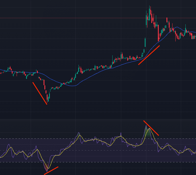
可以看到在均線下行且 RSI 在超賣區升破低點向上時,股價呈現上升的情況;同理,在均線上揚且 RSI 在超買區跌破低點下行時,股價在不久後也隨之下跌。RSI 的開發者 J. W. Wilder 說過,顯示背離的轉換訊號是「RSI 的最大特長」。
找尋背離的重點是,先在 RSI 劃支撐線 / 壓力線,然後價格的部份也同樣畫線。找尋支撐線的兩個谷底、壓力線的兩個山峰。若畫出來的線方向不同,表示出現背離,顯示市場將朝 RSI 所示的方向轉換。
本文使用 Mac 作業系統以及 Jupyter Notebook 作為編輯器。
import os
os.environ['TEJAPI_KEY'] = "your key"
os.environ['TEJAPI_BASE'] = "https://api.tej.com.tw"
import pandas as pd
import numpy as np
import matplotlib.pyplot as plt

from zipline.data import bundles
from zipline.utils.calendar_utils import get_calendar
from zipline.sources.TEJ_Api_Data import get_Benchmark_Return
資料期間從 2021-01-01 至 2023–12–31,利用 get_universe 取得化學生技醫療股票池,並加入化學生技醫療報酬指數 IX0019,作為大盤比較。
from zipline.sources.TEJ_Api_Data import get_universe
start = '2021-01-01'
end = '2023-12-31'
pool = get_universe(start, end, mkt = 'TWSE', stktp_c = '普通股', main_ind_c = 'M1700 化學生技醫療')
print(f'共有 {len(pool)} 檔股票:\n', pool)

start_dt, end_dt = pd.Timestamp(start, tz='utc'), pd.Timestamp(end, tz='utc')
tickers = ' '.join(pool)
os.environ['ticker'] = tickers+' IX0019'
os.environ['mdate'] = start+' '+end
!zipline ingest -b tquant

bundle = bundles.load('tquant')
benchmark_asset = bundle.asset_finder.lookup_symbol('IX0019',as_of_date = None)
Custom Factor 可以讓使用者自行設計所需的客製化因子,於本次案例我們用以處理:
RSI_diff、SMA_diff,詳情請見 Custom Factors)from zipline.pipeline import Pipeline, CustomFactor
from zipline.pipeline.data import TWEquityPricing
from zipline.TQresearch.tej_pipeline import run_pipeline
from zipline.pipeline.filters import StaticAssets
from zipline.pipeline.factors import SimpleMovingAverage, RSI
from zipline.pipeline.mixins import SingleInputMixin
from numexpr import evaluate
from zipline.utils.math_utils import nanmean
from zipline.pipeline.filters import StaticSids
from numexpr import evaluate
from zipline.utils.input_validation import expect_bounded
from zipline.utils.numpy_utils import rolling_window
from numpy import abs, average, clip, diff, inf
# 客製化因子:取得前一個日期和後一個 RSI 的差值,以此取得斜率
class RSI_diff(CustomFactor):
inputs = (TWEquityPricing.close,)
# We don't use the default form of `params` here because we want to
# dynamically calculate `window_length` from the period lengths in our
# __new__.
params = ("rsi_period", "lag_period")
@expect_bounded(
rsi_period=(1, None), # These must all be >= 1.
lag_period=(1, None),
)
def __new__(cls, rsi_period=14, lag_period=2, *args, **kwargs):
return super(RSI_diff, cls).__new__(
cls,
rsi_period=rsi_period,
lag_period=lag_period,
window_length=rsi_period + lag_period + 1,
*args,
**kwargs,
)
def compute(
self, today, assets, out, close, rsi_period, lag_period
):
def rsi(closes):
diffs = diff(closes, axis=0)
ups = nanmean(clip(diffs, 0, inf), axis=0)
downs = abs(nanmean(clip(diffs, -inf, 0), axis=0))
return evaluate(
"100 - (100 / (1 + (ups / downs)))",
local_dict={"ups": ups, "downs": downs},
global_dict={},
out=out,
)
new = np.array(rsi(close[-rsi_period:]))
old = np.array(rsi(close[:-lag_period]))
out[:] = new-old
# 客製化因子:取得前一個日期的均線和後一個均線的差值,以此取得斜率
class SMA_diff(CustomFactor):
def compute(self, today, assets, out, data):
out[:] = ((np.nanmean(data[1:self.window_length], axis=0) -\
np.nanmean(data[0:int(self.window_length)-1], axis=0))).round(4)Pipeline() 提供使用者快速處理多檔標的的量化指標與價量資料的功能,於本次案例我們用以處理:
RSI、SimpleMovingAverage,詳情請見 Pipeline built-in factors)window_length 設置為 14 天,RSI 均線和 SMA 的 window_length 均設置為 10 天。def make_pipeline(rsi_window_length, rsi_slope_wl, sma_window_length):
rsi = RSI(inputs = [TWEquityPricing.close], window_length = rsi_window_length)
rsi_slope = RSI_diff(rsi_period=rsi_window_length, lag_period=rsi_slope_wl)
curr_price = TWEquityPricing.close.latest
sma = SimpleMovingAverage(inputs = [TWEquityPricing.close], window_length = sma_window_length)
sma_slope = SMA_diff(inputs=[TWEquityPricing.close], window_length = sma_window_length + 1)
return Pipeline(
columns = {
"RSI": rsi,
'RSI_based_MA': rsi_slope,
"SMA": sma,
'SMA_slope': sma_slope,
'curr_price': curr_price
},
screen = ~StaticAssets([benchmark_asset])
)
my_pipeline = run_pipeline(make_pipeline(14, 5, 30), start_dt, end_dt)
my_pipeline.head(822).tail(30)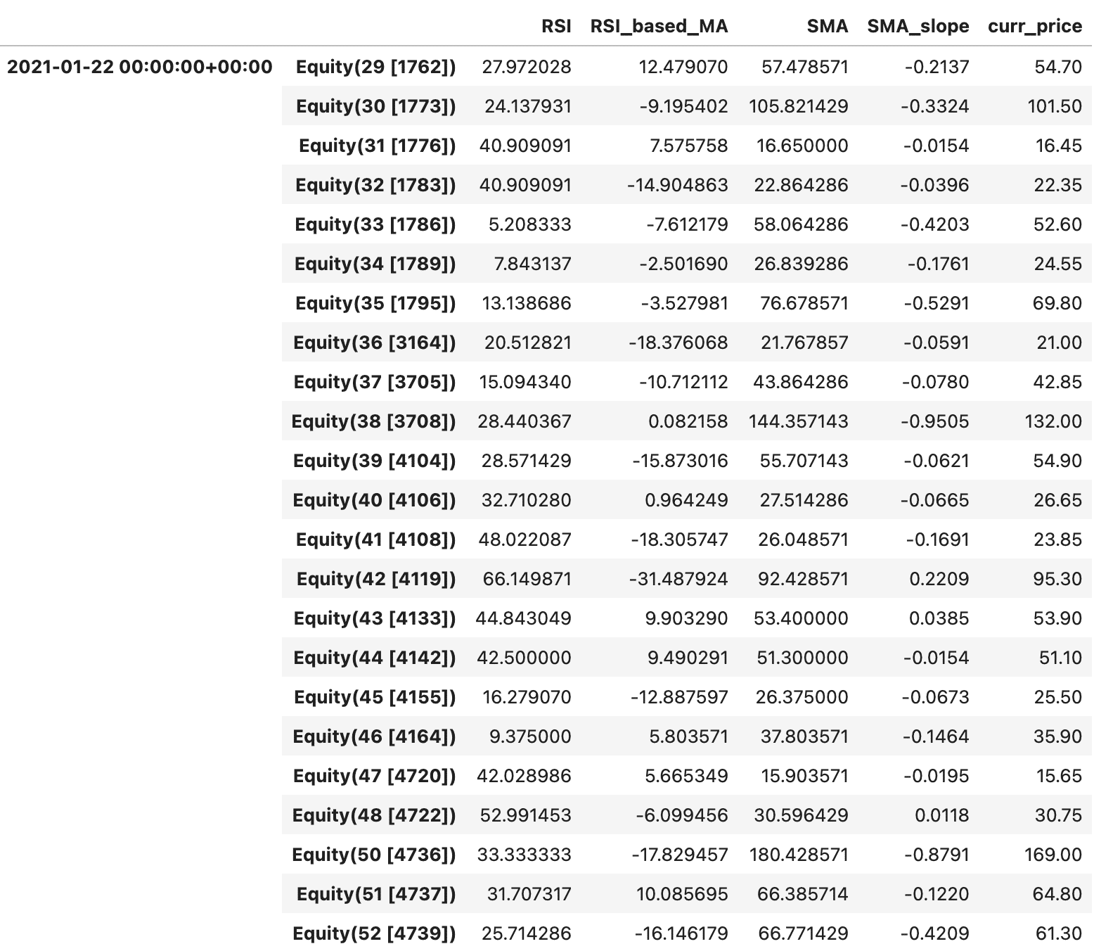
inintialize() 函式用於定義交易開始前的每日交易環境,與此例中我們設置:
from zipline.finance import slippage, commission
from zipline.api import set_slippage, set_commission, set_benchmark, attach_pipeline, order, order_target, symbol, pipeline_output, record

def initialize(context):
    set_slippage(slippage.VolumeShareSlippage())
    set_commission(commission.PerShare(cost = 0.001425 + 0.003 / 2))
    attach_pipeline(make_pipeline(14, 10, 10), 'mystrats')
set_benchmark(symbol('IX0019'))handle_data() 為構建 RSI 均線策略的重要函式,會在回測開始後每天被呼叫,主要任務為設定交易策略、下單與紀錄交易資訊。
接下來將本策略買賣規則在 handle_data() 中建立:
def handle_data(context, data):
    out_dir = pipeline_output('mystrats')
    for i in out_dir.index:
        sym = i.symbol
        rsi = out_dir.loc[i, "RSI"]
        rsi_based_ma = out_dir.loc[i, 'RSI_based_MA']
        sma = out_dir.loc[i, "SMA"]
        sma_slope = out_dir.loc[i, 'SMA_slope']
        curr_price = out_dir.loc[i, 'curr_price']

        cash_position = context.portfolio.cash    # 記錄現金水位
        stock_position = context.portfolio.positions[i].amount    # 記錄股票部位

        buy, sell = False, False

        record(
           **{
                f'price_{sym}':curr_price,
                f'RSI_{sym}':rsi,
                f'RSI_based_MA_{sym}':rsi_based_ma,
                f'SMA_{sym}':sma,
                f'SMA_slope_{sym}': sma_slope,
                f'buy_{buy}':buy,
                f'sell_{sym}':sell
            }
        )

        if stock_position == 0:
            if (rsi <= 30) and (rsi_based_ma > 0) and (sma_slope < 0) and (cash_position >= curr_price * 1000):
                order(i, 1000)
                buy = True
                record(
                    **{
                        f'buy_{sym}':buy
                    }
                )
            else:
                pass
        elif stock_position > 0:
            if (rsi > 45) and (rsi < 55) and (rsi_based_ma > 0) and (sma_slope > 0) and (cash_position >= curr_price * 1000):
                order(i, 1000)
                buy = True
                record(
                    **{
                        f'buy_{sym}':buy
                    }
                )
            elif (rsi >= 70) and (rsi_based_ma < 0) and (sma_slope > 0) and (stock_position > 0):
                order_target(i, 0)
                sell = True
                record(
                    **{
                        f'sell_{sym}':sell
                    }
                )
            else:
                pass
        else:
pass使用 run_algorithm() 執行上述設定的 RSI 均線策略,設置交易期間為 start_time(2021-01-01) 到 end_time(2023-12-31),使用資料集 tquant,初始資金為 5,000,000 元。其中輸出的 results 就是每日績效與交易的明細表。
from zipline import run_algorithm
results = run_algorithm(
    start = start_dt,
    end = end_dt,
    initialize=initialize,
    bundle='tquant',
    analyze=analyze,
    capital_base=5e6,
    handle_data = handle_data
)
results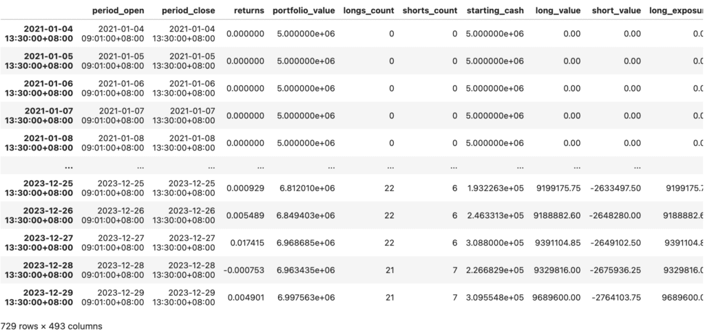
import pyfolio as pf
from pyfolio.utils import extract_rets_pos_txn_from_zipline

returns, positions, transactions = pf.utils.extract_rets_pos_txn_from_zipline(results)
benchmark_rets = results.benchmark_return

# Creating a Full Tear Sheet
pf.create_full_tear_sheet(returns, positions = positions, transactions = transactions,
                          benchmark_rets = benchmark_rets,
                          round_trips=False)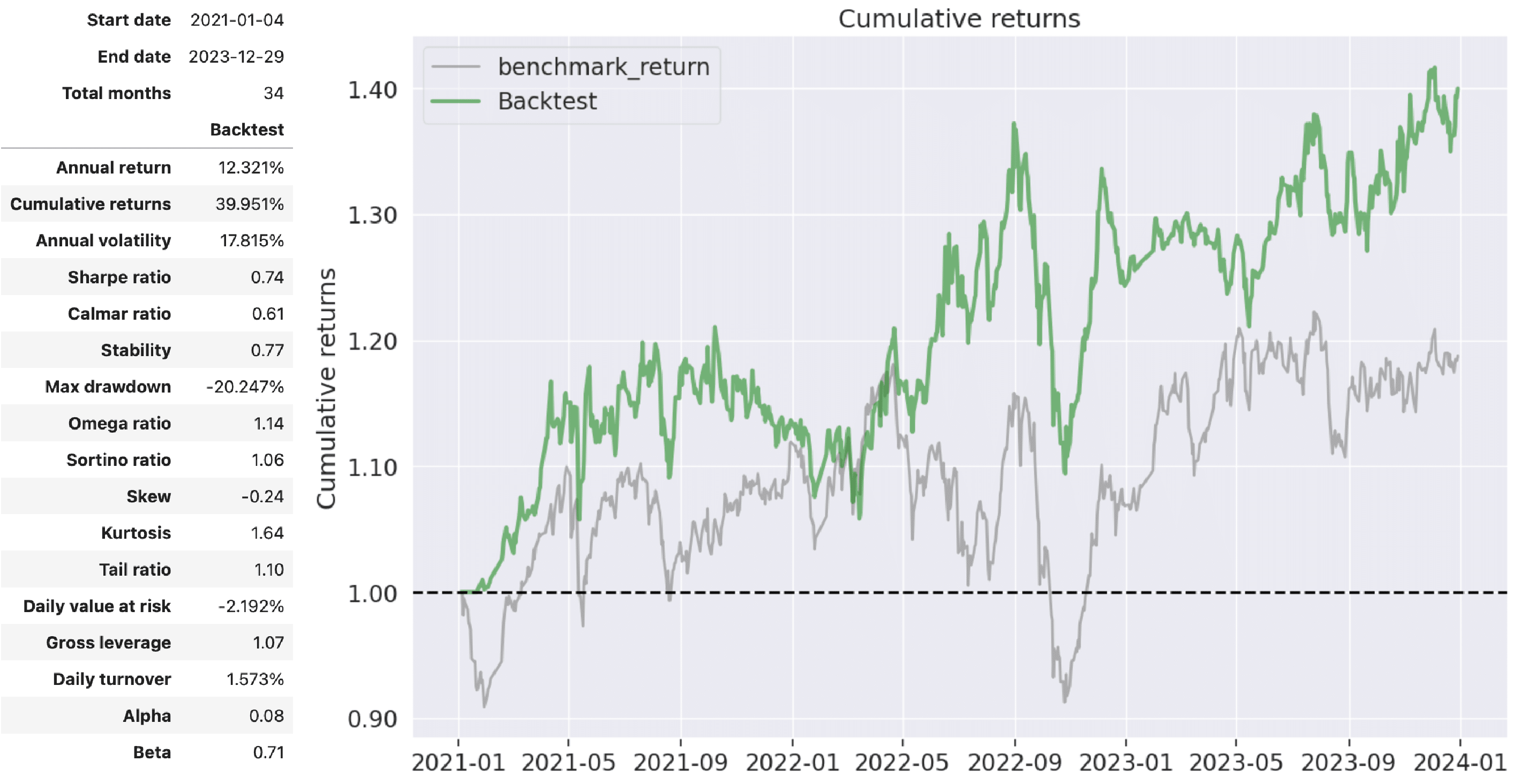
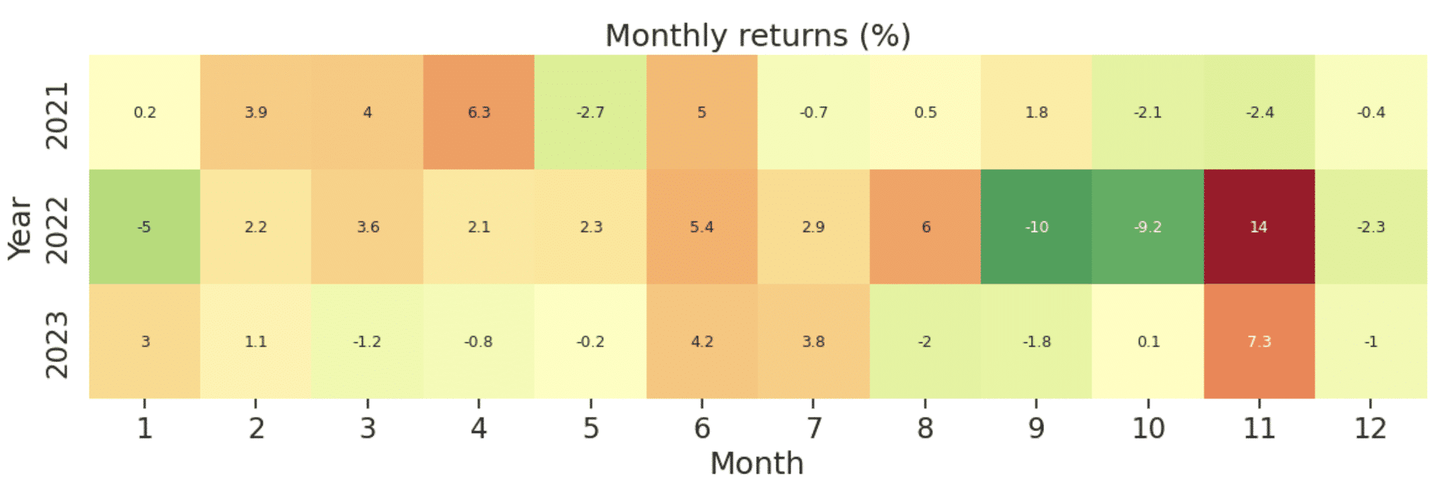
可以看到 RSI 均線策略在這 34 個月中我們獲得了約 12.32% 的年化報酬,累積報酬接近 40%,整體表現也是超越大盤;不過相對來說策略本身依靠股價上下波動反向操作,也使得策略波動性較大,來到 17% 左右;Max drawdown 的部分可以看到大盤在 2022 年因美聯準會升息、新冠疫情等因素導致 Q3、Q4 衰退期表現不佳,RSI 均線策略的報酬率略有下滑。
本次策略使用 RSI 背離提前判斷股價低點,結合簡單移動平均線提供方向性進行反向操作,同理,使用 RSI 均線策略進行做空也是可行的,歡迎投資朋友參考。之後也會持續介紹使用 TEJ 資料庫來建構各式指標,並回測指標績效,所以歡迎對各種交易回測有興趣的讀者,選購 TQuant Lab 的相關方案,用高品質的資料庫,建構出適合自己的交易策略。
溫馨提醒,本次策略僅供參考,不代表任何商品或投資上的建議。