Establish a pairs trading strategy between Evergreen Shipping and Yang Ming Shipping with Python.

Table of Contents
When the market capital is excessively flooded, to avoid systemic risks, investors often establish long and short positions at the same time through asset allocation to eliminate most market risks and obtain stable returns. However, we select Evergreen and Yangming as the stock pair for pairs trading and use a single root test to determine whether the two-level spread has a stationary state. That is, it confirms that Evergreen and Yangming have a cointegration relationship. When the spread deviates, buy undervalued stocks, sell overvalued stocks, and reverse the position to earn the spread when the spread corrects.
Windows OS and Jupyter Notebook
# 基本功能
import pandas as pd
import numpy as np
from arch.unitroot import ADF
import statsmodels.api as sm# 繪圖
import matplotlib.pyplot as plt
plt.rcParams['font.sans-serif'] = ['Microsoft JhengHei']
plt.rcParams['axes.unicode_minus'] = False# TEJ API
import tejapi
tejapi.ApiConfig.api_key = 'Your Key'
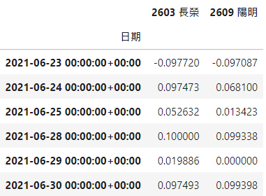
Return Information Data Table: Listed securities with the daily return. Code is ‘TWN/EWPRCD2’.
Import the share price returns of Evergreen and Yang Ming from the TEJ database.
# 匯入資料
stock = tejapi.get('TWN/EWPRCD2',
                   coid = ['2603','2609'],
                   mdate= {'gte': '2019-06-01','lte':'2021-06-30'},
                   opts={'columns':['coid','mdate','roia']},
                   chinese_column_name=True,paginate=True)stock = stock.pivot(index='日期', columns='證券碼', values='日報酬率(%)')
stock.columns = ['2603 長榮','2609 陽明']
stock = stock * 0.01
stock.tail(6)
Step 1. The series of daily stock returns have a stationary state
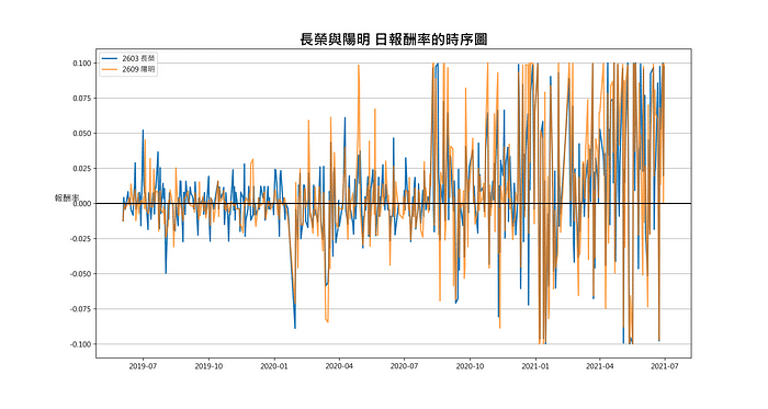
We can see that the two-level daily rate of return fluctuates around 0 from the figure below, and we can confirm that the two-level daily rate of return series has a steady state.
# 長榮與陽明 日報酬率的時序圖
fig = plt.figure(figsize = (15,8))
ax = fig.add_subplot()ax.plot(stock['2603 長榮'] ,linewidth=2, alpha=1)
ax.plot(stock['2609 陽明'] ,linewidth=2, alpha=0.7)
ax.axhline(0,color = 'black')
ax.set_title('長榮與陽明 日報酬率的時序圖' ,fontsize=20 ,fontweight='bold')
ax.legend(['2603 長榮','2609 陽明'],loc='best')
ax.set_ylabel('報酬率', fontsize=12,rotation=0)
ax.grid(axis='y')
Step 2. Calculate the spread of the stock pair
First, We divide the backtest period into the formation and trading periods. When we calculate the spread sequence of the trading period to avoid the forward-looking bias, we use the alpha coefficient value and the beta coefficient value obtained from the linear regression of the spread series in the formation period to calculate the spread series for the trading period.
# 價差
def CointegrationSpread(df,formStart,formEnd,tradeStart,tradeEnd):
    formX = df[(df.index >= formStart) & (df.index <= formEnd)]['2603 長榮']
    formY = df[(df.index >= formStart) & (df.index <= formEnd)]['2609 陽明']
    tradeX = df[(df.index >= tradeStart) & (df.index <= tradeEnd)]['2603 長榮']
    tradeY = df[(df.index >= tradeStart) & (df.index <= tradeEnd)]['2609 陽明']

    results = sm.OLS(formY,sm.add_constant(formX)).fit()
    spread = tradeY - results.params[0] - results.params[1] * tradeX
    return spreadSpread_2020_10_12 = CointegrationSpread(stock,'2019-06-01','2020-06-30','2020-10-01','2020-12-31')
Spread_2021_01_03 = CointegrationSpread(stock,'2020-01-01','2020-12-31','2021-01-01','2021-03-30')# 對兩檔股價的價差序列做定態性檢定
adfSpread = ADF(Spread_2021_10_12, trend='n')
print(adfSpread.summary().as_text())
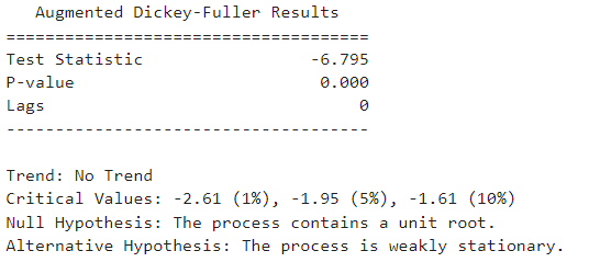
We see in the below figure that we can reject the null hypothesis at the 1% significance level, indicating that the 2021_10_12 spread series is stationary. The daily return series of Evergreen and Yangming have a cointegration relationship.
We formulate trading strategies based on the opening and closing points,
Spread_2021_01_03 = Spread_2021_01_03.to_frame()
Spread_2021_01_03.columns = ['價差']Spread_2021_01_03['開倉平倉區間'] = \
    pd.cut(Spread_2021_01_03['價差'] ,
           (float('-inf') ,mu-2.5*sd ,mu-1.5*sd ,mu-0.2*sd ,
            mu+0.2*sd ,mu+1.5*sd ,mu+2.5*sd ,float('inf')) ,labels=False)-3Spread_2021_01_03['交易訊號'] = \
    np.select([(Spread_2021_01_03['開倉平倉區間'].shift() == 1) &
               (Spread_2021_01_03['開倉平倉區間'] == 2),

               (Spread_2021_01_03['開倉平倉區間'].shift() == 1) &
               (Spread_2021_01_03['開倉平倉區間'] == 0),

               (Spread_2021_01_03['開倉平倉區間'].shift() == 2) &
               (Spread_2021_01_03['開倉平倉區間'] == 3),

               (Spread_2021_01_03['開倉平倉區間'].shift() == -1) &
               (Spread_2021_01_03['開倉平倉區間'] == -2),

               (Spread_2021_01_03['開倉平倉區間'].shift() == -1) &
               (Spread_2021_01_03['開倉平倉區間'] == 0),

               (Spread_2021_01_03['開倉平倉區間'].shift() == -2) &
               (Spread_2021_01_03['開倉平倉區間'] == -3)],

              [-2,2,3,1,-1,-3],default = 0)position = [Spread_2021_01_03['交易訊號'][0]]
ns = len(Spread_2021_01_03['交易訊號'])Spread_2021_01_03['倉位情況'] = pd.Series(position,index=Spread_2021_01_03.index)
Spread_2021_01_03['倉位情況'] = Spread_2021_01_03['倉位情況'].shift() # 隔天開盤才進場Spread_2021_01_03 = Spread_2021_01_03.join(stock)
Spread_2021_01_03['策略報酬率'] = \
    np.select([Spread_2021_01_03['倉位情況'] == 1,
               Spread_2021_01_03['倉位情況'] == 0,
               Spread_2021_01_03['倉位情況'] == -1],
              [Spread_2021_01_03['2609 陽明'] * -1 + Spread_2021_01_03['2603 長榮'] * 1,
               0,
               Spread_2021_01_03['2609 陽明'] * 1 + Spread_2021_01_03['2603 長榮'] * -1], default=np.nan)Spread_2021_01_03['累積報酬率'] = (Spread_2021_01_03['策略報酬率'] + 1).cumprod() -1
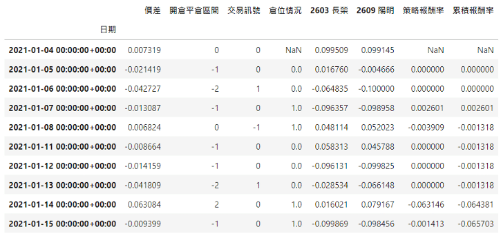
Spread_2021_01_03.head(10)
We complete the above strategy and present the strategy’s cumulative return and a maximum drawdown in the graph below.
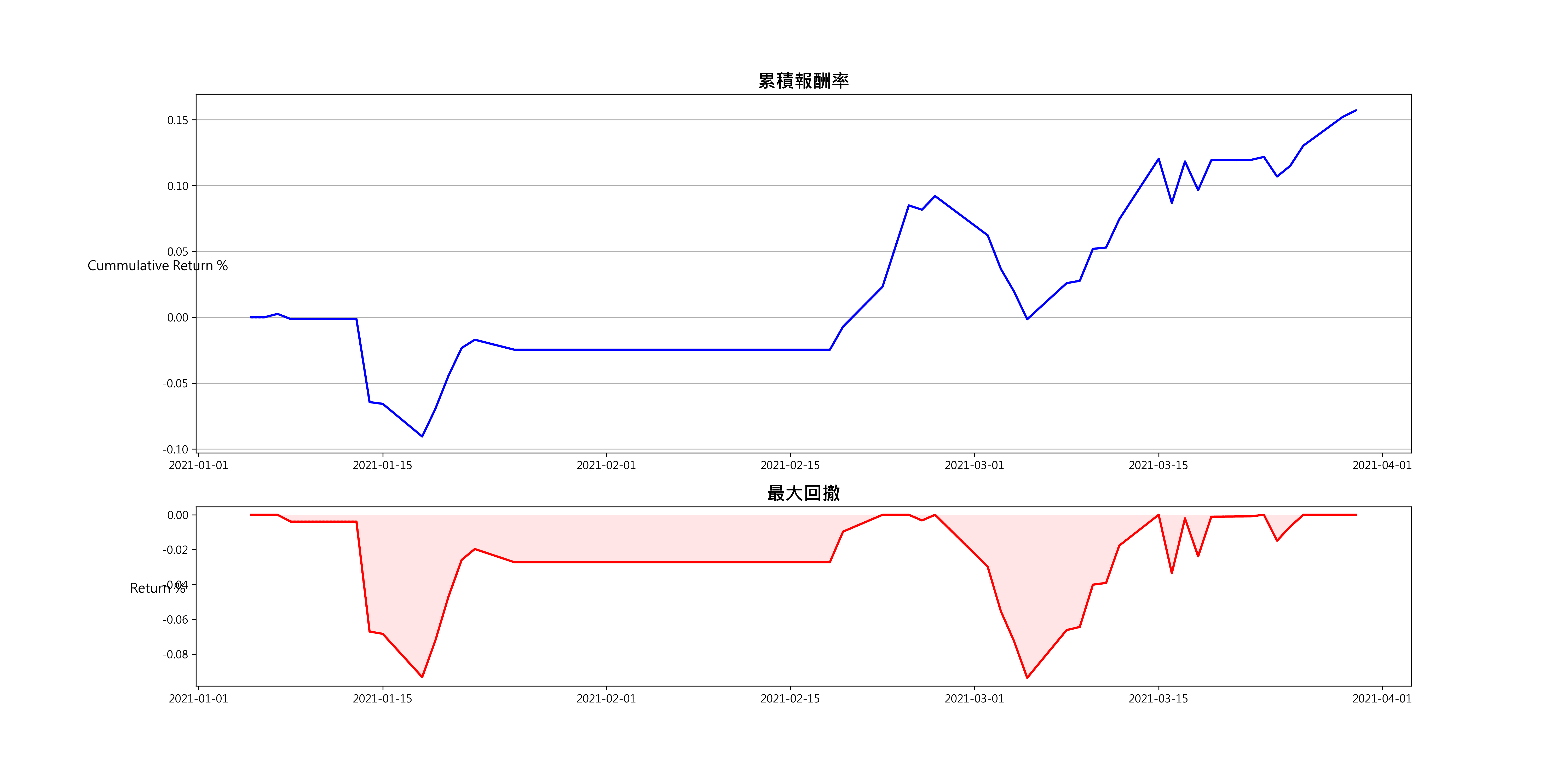
From the maximum drawdown chart, We can find that the maximum drawdown of the two pairs trade has fallen below 8% in a row, which means that the strategy’s stop-loss mechanism is not very good, or the μ mean and σ parameters are out of order. In the future, you can try to lower the standard of 2.5σ or calculate the μ mean and σ standard deviation of the formation period spread series in a rolling method because the volatility of maritime stocks in the first half of 2021 is extremely high. As a result, the trading period fell in 2021. From January to March 2020, the formation period is from January to December 2020.
The content of this webpage is not an investment device and does not constitute an offer or solicitation to offer or recommendation of any investment product. It is for learning purposes only and does not consider your individual needs, investment objectives, and specific financial circumstances. Investment involves risk. Past performance is not indicative of future performance. Readers are requested to use their independent thinking skills to make investment decisions independently. The author will not be involved if losses are incurred due to relevant suggestions.

Subscribe to newsletter