[TQuant From 0 to 1 - Day 5] Introduction to Order Placement Methods in the TQuant Lab Backtesting System

Introduction

In TQuant backtesting and live trading, order functions serve as the central link between strategy logic and capital management. Choosing the right order method not only makes the code cleaner and easier to read but also improves the efficiency of risk control and portfolio rebalancing.

TQuant provides order functions across three dimensions — share quantity, capital amount, and portfolio weight. For each dimension, there are two variants: a basic order and a target order. In total, this gives us six order placement methods. In the following sections, we will explain the features, parameters, and recommended applications of each.

How to Use in Practice

As explained in previous articles, order functions are primarily implemented inside the handle_data function, where trading logic is defined. During backtesting, the run_algorithm function executes a loop that evaluates the conditions on each trading day to determine whether orders should be placed.

This design allows you to set very detailed order logic, enabling strategies that can better adapt to real-world trading scenarios.

Introduction to Order Functions

order(asset, amount) — Order by Share Quantity

Function: Buy or sell directly with a specified number of shares. Suitable when precise control of trade quantities is required.

Parameters:

• asset: Target asset (e.g., symbol('Ticker'))
• amount: Number of shares (positive = buy, negative = sell)

Use Case Suggestion: When you know the fixed number of shares for each trade, or need to operate within a specific share range, order is the most straightforward choice.

order_target(asset, target_amount) — Order to Target Share Quantity

Function: Automatically calculates (target shares − current shares) and places an order to adjust holdings to the target. Suitable for position-adjustment strategies that are guided by shareholding targets.

Parameters:

• asset: Target security
• target_amount: Final shareholding quantity

Use Case Suggestion: If the requirement is to “adjust to a fixed number of shares,” this function saves the effort of manually calculating the difference.

order_value(asset, value) — Order by Capital Amount

Function: Buy or sell with a specified capital amount. The system estimates the number of shares based on the current day’s price. Suitable for operations measured by capital allocation.

Parameters:

• asset: Target security
• value: Buy/sell amount (positive = buy, negative = sell)

Use Case Suggestion: When the strategy involves a fixed monetary amount per trade, or when allocating based on a proportion of total portfolio capital, order_value is the most intuitive.

order_target_value(asset, target_value) — Order to Target Market Value

Function: Adjust holdings to reach the specified market value (target value − current value). Convenient for rebalancing at the market-value level.

Parameters:

• asset: Target security
• target_value: Final holding market value

Use Case Suggestion: In multi-asset portfolios, when strict market-value rebalancing is required, this function is particularly useful.

order_percent(asset, percent) — Order by Portfolio Weight

Function: Buy or sell based on a proportion of the portfolio’s net value. For example, 0.1 means buying a position equal to 10% of net portfolio value.

Parameters:

• asset: Target security
• percent: Proportion of portfolio (positive = buy, negative = sell)

Use Case Suggestion: When dynamically adjusting asset weights without needing exact shares or capital amounts, order_percent is the simplest option.

---

order_target_percent(asset, target_percent) — Order to Target Portfolio Weight

Function: Adjusts the asset position to reach a target portfolio weight (target weight − current weight). Ensures strict portfolio rebalancing.

Parameters:

• asset: Target security
• target_percent: Final target weight (range: −1.0 to 1.0)

Use Case Suggestion: In multi-asset portfolios or rotation strategies, order_target_percent is the most direct and intuitive tool for rebalancing.

Practical Exercise

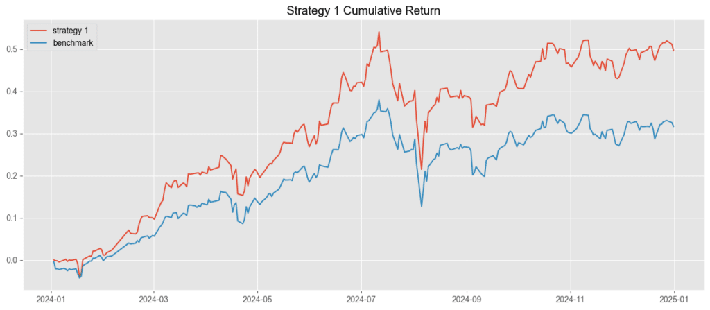
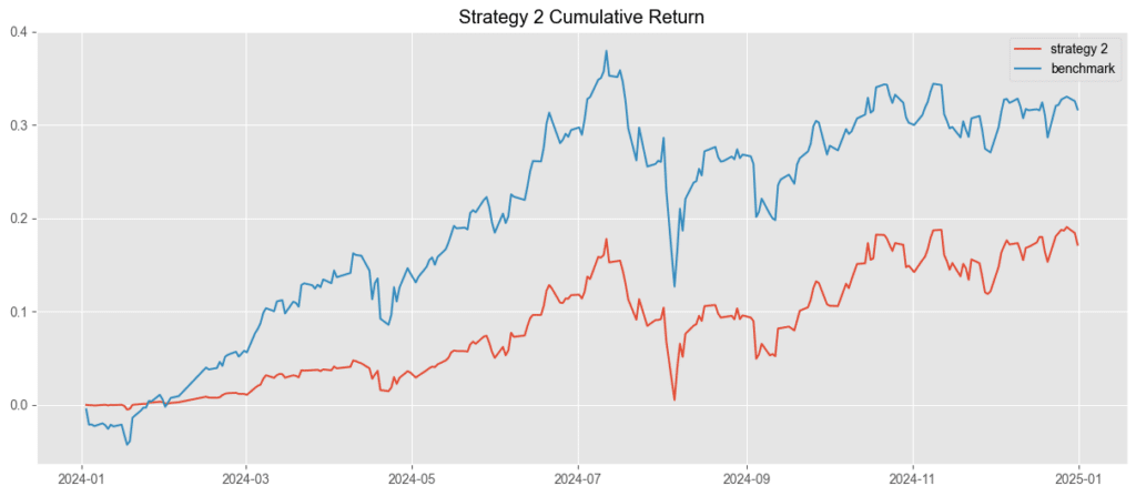
By combining the content from TQuant Day 4, we can integrate the four major backtesting frameworks with the newly learned order placement methods to build a simple investment strategy.

For clarity, we will demonstrate two straightforward strategies:

1. Buy-and-Hold 0050
   At the start of the backtest, buy 0050 and hold it until the end of the testing period.
2. Dollar-Cost Averaging (DCA) on 0050
   Invest 10,000 NTD every 30 trading days until the allocated capital is fully used.

First, we need to import the backtesting data. This part will be explained in detail in the next article. For now, just understand that this step involves importing the stock data required for trading into the backtesting system.

Code snippet for importing backtest data:
In this example, the backtesting period is set from 2023-12-31 to 2024-12-31, covering approximately 252 trading days. Readers can add any stock symbols they wish to trade into the pool list, and their price–volume data will be imported into the backtesting system.

Display backtest results and visualize with charts

Strategy 2

Conclusion

In this article, we introduced six order placement methods in Zipline, each with its own applicable scenarios, advantages, and limitations. The choice between precise share quantities, capital amounts, or portfolio weights should be guided by strategy logic and risk management requirements. Mastering the correct order functions not only streamlines backtesting code but also ensures accuracy in trade execution, thereby improving both the efficiency and quality of strategy development. Wishing you greater success in quantitative research and live trading applications!

We also welcome investors to explore further. In the future, we will continue to introduce how to build various indicators using the TEJ database and backtest their performance. Readers interested in trading backtests are encouraged to consider TQuant Lab’s solutions, which leverage high-quality databases to help you develop trading strategies tailored to your needs.

Disclaimer: This analysis is for reference only and does not constitute any product or investment advice.

Next Article – [TQuant From 0 to 1 – Day 6] (link coming soon)

Further Reading

【TQuant : From 0 to 1 – Day 1】 Your Gateway to Quantitative Trading: Become a Quant Expert with TQuant Lab, No Experience Needed!

【TQuant : From 0 to 1 – Day 2】 Avoid the Invisible Killers of Quantitative Trading: Use TQuant Lab to Precisely Manage Commission and Slippage, Giving Your Strategies the Edge!

【TQuant from 0 to 1 – Day 3】Building a Comprehensive Investment Data Perspective: Stock Pool Screening and Data Retrieval with TejToolAPI

【TQuant : From 0 to 1 – Day 4】 Core Architecture of Backtesting: What are the key settings for Initialize?

Related Links

• TQuant Lab GitHub
• TQuant Lab Official Website