
Photo by Chris Liverani on Unsplash
Table of Contents
In investing, factor strategies are an indispensable tool, whether you’re an experienced professional trader or a newcomer to the market. The essence of factor strategies lies in leveraging quantitative analysis to distill the market’s complex movements into key driving forces. These strategies help investors capture market trends and enhance investment efficiency. Factors can analyze market behavior and serve as a reliable foundation for asset allocation and risk management strategies.
This series of articles uses Alphalens to examine the application and effectiveness of various factors in the market. In previous articles, we analyzed “foreign capital factors,” exploring how foreign investments influence the market. This article will focus on “value factors,” examining valuation-related indicators that reveal intrinsic value and affect long-term returns. The final article will discuss “price-volume factors,” delving into the relationship between price and trading volume and uncovering investment opportunities.
If you want to conduct similar factor analyses, you can use the alphalens-tej tool within TQuant Lab. This tool not only integrates TEJ data but also eliminates tedious data processing, allowing you to easily assess factor performance and further support the development of investment strategies.
In the investment market, value factors are essential tools for measuring the intrinsic value of assets. They are typically associated with a company’s fundamental indicators, such as Price-to-Earnings ratio (P/E), Price-to-Book ratio (P/B), and Dividend Yield. These metrics reflect the market’s expectations of a company’s future growth and profitability and are widely used to determine whether an asset is undervalued or overvalued. By applying value factors in investment strategies, investors can analyze valuation differences across companies and potentially achieve excess returns by holding relatively undervalued assets.
Factors Used in This Article:
Calculation Formulas:
Calculation Formulas:
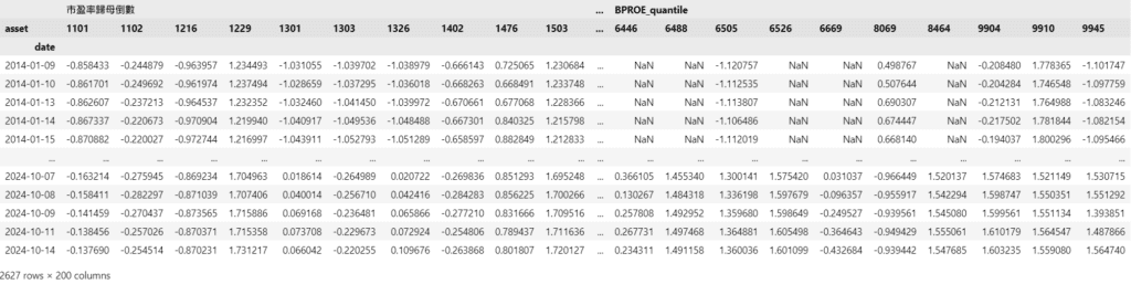
Company Market Capitalization Divided by Parent Company Net Profit (Inverse)
The PB and market capitalization data used in this article are sourced from the TEJAPI “Trading Data – Stock Price Data” table (TWN/APIPRCD), specifically the columns “Price-to-Book Ratio” and “Individual Stock Market Value (NTD).”
The ROE and parent company net profit data are sourced from the TEJAPI “Financial Data – CPA-Audited Financial Data” table (TWN/AINVFQ1), specifically the columns “Sustainable ROE” and “Parent Company Net Profit.”
The financial data for ROE and parent company net profit are based on a trailing twelve months (TTM) period.
The Alphalens-tej package in TQuant Lab is a Python toolkit designed explicitly for factor analysis. Its primary function is to help investors review and evaluate factor performance, enabling the creation of more effective factor strategies. For a detailed introduction, refer to the Alphalens.ipynb notebook.
In quantitative investing, factors are indicators used to explain and predict asset returns. Common examples include price-to-earnings ratios, price momentum, and trading volume.
Alphalens offers a suite of powerful visualization tools and metrics, such as:
These features allow a deeper understanding of a factor’s predictive power and stability. Using Alphalens, investors can easily analyze the performance of various factors under different market conditions and identify the most suitable combinations for their strategies.
Alphalens integrates seamlessly with TEJ data, making it especially suitable for conducting factor backtesting and visualization using TQuant Lab. This integration significantly enhances the convenience and efficiency of factor research.
Due to space limitations, this section only calculates the factor’s IC (Information Coefficient) and IR (Information Ratio, risk-adjusted IC). It generates bar charts of the average returns for each factor quantile. The sample period for this article spans from 2014 to 2024, and the stock universe consists of the top 100 most extensive market capitalization stocks listed on the exchange.
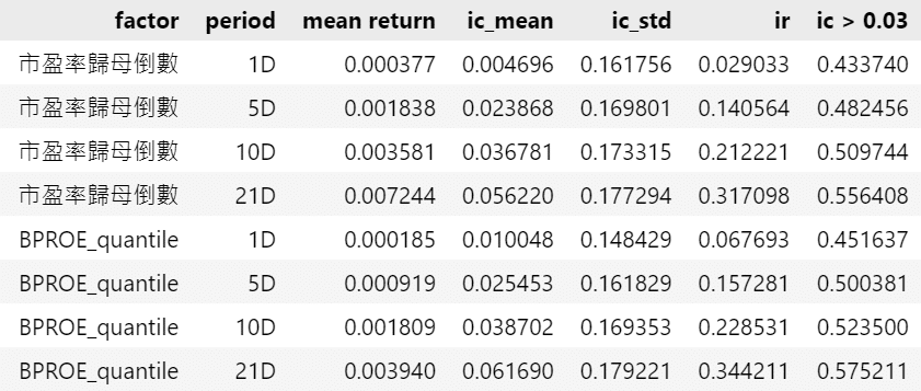
The table “IC, IR Values, and Weighted Average Returns of Factor Values” shows that these two factors underperformed in terms of IC and IR across most holding periods. Generally, a factor with an IC greater than 0.05 and an IR greater than 0.3 is considered to have strong predictive power. However, these factors only met this standard during the 21-day holding period, indicating that their correlation with asset returns becomes more apparent over longer holding periods. Additionally, the table shows that the overall predictive ability of “BPROE_quantile” surpasses the “Inverse P/E Ratio” as its IC and IR values are consistently higher.
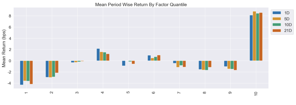
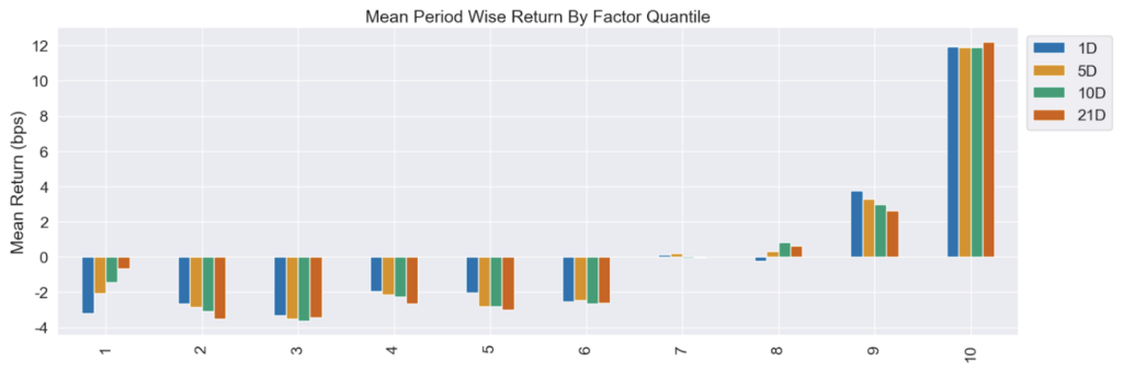
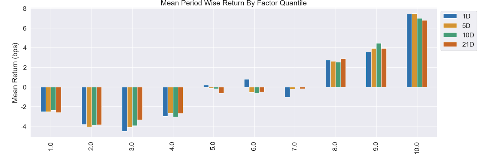
In the “Mean Return by Factor Quantile Bar Chart,” “BPROE_quantile” does not exhibit clear monotonicity, especially with inconsistent performance in the middle quantiles, suggesting a lack of pronounced monotonicity. In contrast, the “Inverse P/E Ratio” factor shows a stable and significant upward trend in higher quantiles, though its monotonicity is less evident in the lower quantile groups. Thus, the average return monotonicity of both factors is not sufficiently consistent.
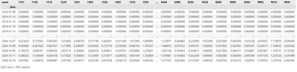
In the previous section, we observed that both “BPROE_quantile” and “Inverse P/E Ratio” achieved more favorable IC values over more extended holding periods. However, the monotonicity across different quantiles was not consistent. This section will attempt to synthesize these two factors and explore whether their predictive power can be further enhanced through the combination.
When synthesizing multiple factors, assigning appropriate weights to each factor is essential since their explanatory power for future returns can vary. Proper weighting enhances predictive accuracy and stability.
In this article, rank IC_IR is used to calculate factor weights. Rank IC_IR is determined by dividing the IR ratio of each factor over the past month by the total IR ratios of the two factors. This method of weight calculation, based on risk-adjusted IC, assigns greater weights to factors with more substantial predictive power and stability.
We applied a lag (shift) to the final weight data to simulate the signal delay in actual trading. By shifting the weights by one day, we ensured that only prior-period data was used, avoiding the use of future information in the model.
The method for calculating the composite factor involves weighting each individual factor based on its assigned weight and then computing a weighted average to create a composite factor that represents the overall factor effect.
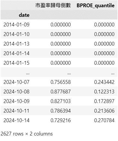
As with single-factor analysis, we similarly import the new composite factor data into Alphalens.
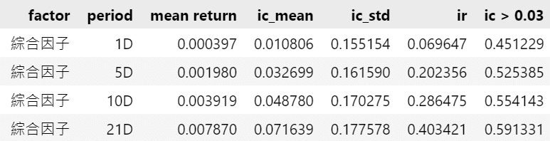
The table “IC, IR Values, and Weighted Average Returns for the Composite Factor” shows that the composite factor slightly outperforms the original individual factors in terms of IC, IR, and average returns. Notably, the performance significantly improved during the 21-day holding period, with IC exceeding 0.07 and IR surpassing 0.4.
Furthermore, from the “Mean Return by Quantile Bar Chart”, it is evident that the composite factor demonstrates a more pronounced monotonic increasing effect across the quantiles. Compared to using individual factors alone, the composite factor exhibits more excellent stability and superior performance.
Through this analysis, we demonstrated how to use Alphalens to evaluate the performance of value factors and apply them to practical investment strategies. The value factors analyzed were “Inverse P/E Ratio” and “BPROE_quantile.” Based on the IC and IR results from single-factor analysis, the predictive ability of these factors was significant only during the 21-day holding period.
We synthesized the two value factors using weighted averages in the composite factor analysis. The results showed that the composite factor improved predictive power and monotonicity, with the most notable performance during the 21-day holding period. Based on these findings, future strategies could consider using the composite factor with a 21-day holding period.
Overall, this article presented a complete process, from single-factor analysis to constructing and backtesting composite factors. For future applications, consider incorporating additional value factors and experimenting with different weighting methods to enhance the efficiency of factor synthesis. Additionally, transaction costs, such as slippage and fees, should be included to evaluate the practical feasibility of the strategy further. With these improvements, multi-factor strategies will be better equipped to handle market volatility and consistently generate value in dynamic market conditions.
Start Building Portfolios That Outperform the Market!
