
Table of Contents
You’ll inevitably encounter numerous factor strategies, whether you are an experienced trader or a beginner. By selecting factors that closely correlate with market performance, investors can more effectively predict asset returns and find stable sources of income in uncertain market environments. The essence of factor strategies lies in simplifying complex market phenomena into a few quantifiable drivers, helping us understand capital flows and risk distribution. These factors reveal the roots of market volatility and provide practical decision-making tools for investors.
This series of articles will use Alphalens to explore several key factors, gradually analyzing their impact on market performance. The first article focuses on “foreign capital,” examining the effects of foreign capital flows into the market. Next, we’ll delve into “value factors,” studying how they reflect a company’s intrinsic value. Finally, the last article will analyze “price-volume factors,” uncovering the interplay between price and trading volume.
If you’re interested in conducting similar factor analyses, you can use the alphalens-tej tool in TQuant Lab. By seamlessly integrating TEJ data and eliminating the need for complex data processing, this tool enables you to quickly evaluate factor performance and further support the development of your investment strategies.
In China’s A-share market, “northern-bound funds,” entering the Chinese market through the Shanghai-Hong Kong Stock Connect and Shenzhen-Hong Kong Stock Connect, are regarded as direct indicators of foreign investors’ sentiment toward the Chinese market. These capital flows are often used to monitor market trends and have demonstrated significant influence in related studies. Consequently, northern-bound factors receive considerable attention and application in the Chinese market.
When analyzing northern-bound factors in Taiwan’s stock market, we can observe the changes in foreign holdings across different industries or individual stocks. Foreign investors account for a relatively high proportion of trading volume in the Taiwan market and have a notable impact on market movements. Due to the substantial scale of foreign capital, their buying and selling activities often drive short-term market fluctuations. This is particularly evident in specific industries or leading stocks, where these activities better reflect foreign investors’ preferences and capital flows. By tracking the changes in foreign capital factors, we can more accurately identify trends for asset allocation and even capture early warning signals of market risks.
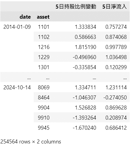
Factors Used in This Article:
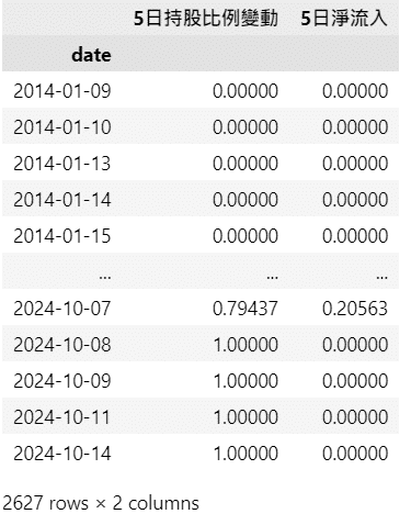
5-Day Change in Foreign Ownership Ratio
5-Day Net Inflows
Data Source:
The data used in this article is sourced from the TEJAPI “Transaction Data — Chip Data (Daily)” table (TWN/APISHRACT). The fields utilized are “foreign ownership ratio” and “foreign buying amount (in TWD).”
The Alphalens-tej package in TQuant Lab is a Python toolkit for factor analysis. Its core functionality assists investors in reviewing and evaluating factor performance, thereby formulating more effective factor strategies. For detailed instructions, refer to Alphalens. ipynb.
In quantitative investing, factors are indicators used to explain and predict asset returns. Common factors include the price-to-earnings ratio (P/E), price momentum, trading volume, etc.
Alphalens provides a series of powerful visualization tools and metrics, such as:
These features help investors better understand a factor’s predictive power and stability. With Alphalens, investors can quickly analyze the performance of various factors under different market conditions and identify the factor combinations or strategies most suitable for them.
Furthermore, Alphalens integrates seamlessly with TEJ data, making it ideal for conducting factor backtesting and visualization analysis using TQuant Lab. This integration dramatically enhances the convenience and efficiency of factor research.
Due to space constraints, this section focuses only on calculating the factor’s IC (Information Coefficient) and IR (Information Ratio, i.e., risk-adjusted IC) and plotting bar charts of the average returns for each factor quantile.
The data sample period used in this article spans from 2014 to 2024, and the stock pool consists of the top 100 market-cap stocks among all listed companies.
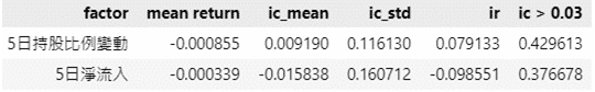
Mean Return
IC Mean
IC Std
IR (Information Ratio)
IC > 0.03
Based on the table “IC, IR Values, and Average Returns for Each Factor,” neither of these factors demonstrates strong IC or IR values. Generally, a good factor should have an IC greater than 0.05 and an IR greater than 0.3. Therefore, these two factors show a low correlation with asset returns and need more stable predictive ability.
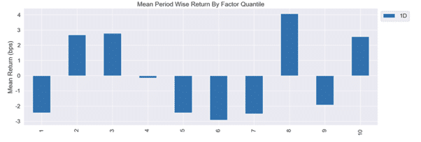
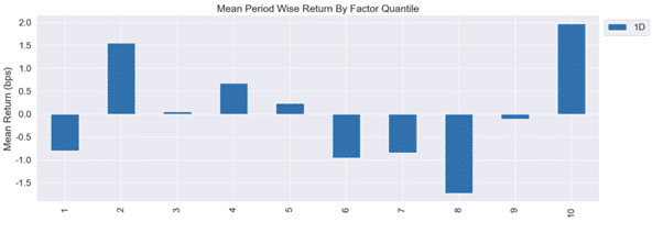
The “Average Returns by Factor Quantile Bar Chart “ also shows that these two factors are unable to effectively predict or indicate asset return trends. Typically, in the bar chart, we aim to see monotonicity in the factor, meaning that larger factor values correlate with higher returns or smaller factor values correlate with lower returns. Factors with this characteristic can support the construction of investment strategies with more stable and consistent returns.
In the previous section, we observed that the predictive effectiveness of the “5-day holding proportion change” and “5-day net inflow” factors was suboptimal. Therefore, this section will attempt to synthesize these two factors and examine whether the predictive power improves after synthesis.
When synthesizing multiple factors, assigning appropriate weights to each factor is crucial due to their varying explanatory power for future returns. Proper weighting enhances both the predictive performance and stability of the composite factor.
In this article, rank IC_IR is used to calculate factor weights. The rank IC_IR is determined by dividing the IR ratio of an individual factor (calculated over the past month) by the sum of the IR ratios for all factors. This provides the relative weight of each factor. Based on risk-adjusted IC, this weighting method assigns greater weight to factors with higher predictive power and stability.
To simulate the delay of factor signals in real-world trading, the final weight data is lagged (shifted) by one day. This ensures that only data from the previous period is used, thereby avoiding the use of future information in the model.
This approach aligns the synthesized factor with practical trading scenarios, improving its robustness and applicability in real-world investment strategies.
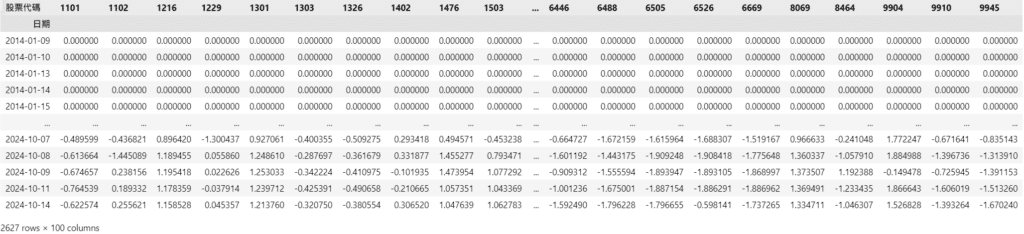
Calculating the composite factor involves generating a single composite factor by taking a weighted average of each factor based on its assigned weight, representing the overall effect of all aspects.
Detailed Steps:
Using this method, the composite factor reflects the relative significance of the individual factors and their collective predictive power, enhancing stability and effectiveness in multi-factor strategies.
Similar to single-factor analysis, we will also import the new composite factor data into Alphalens for evaluation.
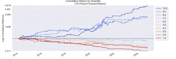
Due to the calculation method of cumulative returns in Alphalens, only the cumulative returns for a 1-day holding period are presented in the line chart. These charts show that the composite factor’s predictive power significantly surpasses that of the individual factors before synthesis.
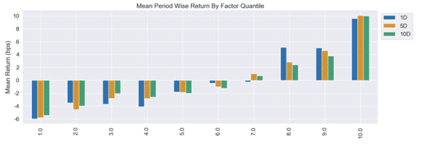
The results show that the 10th quantile achieves the highest returns, while the 1st quantile has the lowest returns. Furthermore, the returns across quantiles exhibit a clear monotonic increasing trend.
Based on these findings, we can further explore constructing a long-short hedge portfolio by going long on stocks in the 10th and shorting stocks in the 1st quantile. This approach aims to maximize returns through effective portfolio hedging.
Through the analysis in this article, we demonstrated how to use Alphalens to evaluate factor performance and apply it in practical investment strategies. Initially, the IC and IR analyses of single factors revealed that the “5-day holding proportion change” and “5-day net inflow” factors performed poorly in predicting asset returns. The quantitative results also indicated a need for more stable monotonicity, making constructing effective long-short hedge strategies challenging. However, we observed a significant improvement in predictive power by synthesizing these factors into a composite factor.
In the composite factor analysis, a clear monotonic relationship between factor values and asset returns was evident, with higher quantiles achieving higher average returns. This monotonicity makes the composite factor well-suited for long-short hedge strategies, enhancing investment portfolios’ stability and return potential. Overall, this article illustrated the process from single-factor analysis to composite factor construction and backtesting, strengthening factor predictive power while reducing strategy risk to some extent.
In the future, practical applications could explore more advanced factor integration methods and alternative weight calculation approaches. Additionally, incorporating considerations such as slippage and transaction costs would further assess the strategy’s real-world feasibility. With these refinements, multi-factor strategies will be better equipped to adapt to market volatility and consistently create value in dynamic market environments!
Start Building Portfolios That Outperform the Market!
