Key Highlights of This Article

Introduction to Alphalens and Price-Volume Factors
Synthesizing Price-Volume Factors and Analyzing Their Performance with Alphalens
Table of Contents
In investment decision-making, price-volume factors are essential for investors to gain insights into market behavior. The relationship between price and trading volume supply and demand dynamics of an asset also reveals capital flows and shifts in market sentiment. These factors play a crucial role in capturing short-term opportunities and identifying potential risks in asset allocation.
This article focuses on price-volume factors, exploring how these factors reflect the dynamic changes in assets and leveraging the Alphalens tool to analyze their performance and practical applications in the market. We will first introduce the concept and design logic of price-volume factors and then use alphabets-tej for analysis to evaluate their explanatory power and stability in predicting asset returns.
In this series of articles, we have previously analyzed foreign capital and value factors, discussing the impact of foreign capital flows on the market and how valuation-related indicators affect long-term returns. This article serves as the final part of the series, further enhancing our comprehensive understanding of factor strategies and helping investors effectively utilize price-volume factors to capture market trends.
To conduct similar factor analyses, you can leverage the alphabets-tej tool in TQuant Lab. This tool not only integrates TEJ data but also eliminates the cumbersome data processing steps, allowing you to efficiently examine factor performance and further support the development of investment strategies.
In the investment market, price-volume factors are essential for uncovering the relationship between asset prices and trading volume. They are often associated with key market dynamics indicators, such as trading volume, volume change rate, and price momentum. These indicators reflect the intensity of market demand for an asset, capital flows, and overall market sentiment.
Price-volume factors are widely used to identify short-term opportunities and assess the persistence of trends. When applied to investment strategies, they allow investors to analyze the interaction between price and trading volume across different assets. By capturing assets with high trading volume or strong price momentum, investors can achieve excess returns and improve investment efficiency.
Calculation formula:
Calculation formula:
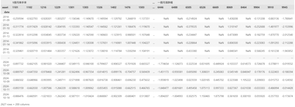
The closing price and trading volume data used in this study are sourced from the TEJAPI “Trading Data – Stock Price Data” table (TWN/APIPRCD), specifically from the “Closing Price” and “Trading Volume (in thousand shares)” columns.
The Alphalens-tej package in TQuant Lab is a Python toolkit for factor analysis. Its core functionality is to help investors examine and evaluate factor performance, enabling them to develop more effective factor strategies. For a detailed introduction, you can refer to Alphalens.ipynb.
In quantitative investing, factors are indicators used to explain and predict asset returns. Common factors include price-to-earnings ratio (P/E ratio), price momentum, and trading volume.
Alphalens provides a set of visualization tools and performance metrics, including:
These tools help us better understand the predictive power and stability of factors. Using Alphalens, investors can quickly analyze the performance of various factors under different market conditions and identify the most suitable factor combinations for their strategies. Additionally, Alphalens is well integrated with TEJ data, making it particularly useful for conducting factor backtesting and visualization within TQuant Lab, thus enhancing the efficiency and convenience of factor research.
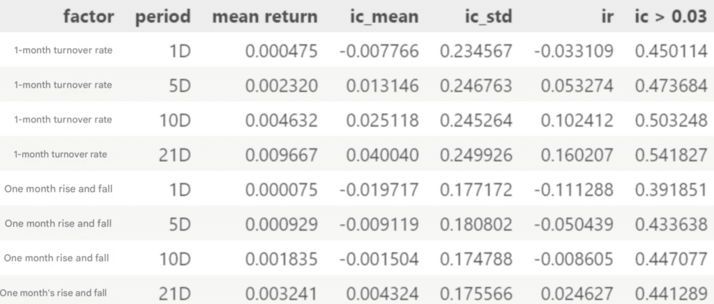
Due to space limitations, this section will focus only on calculating the Information Coefficient (IC) and information Ratio (IR, which is the risk-adjusted IC) and plotting bar charts of the mean return by factor quantile.
The sample period used in this study spans from 2014 to 2024, and the stock universe consists of the top 100 most extensive market-cap stocks listed on the exchange.
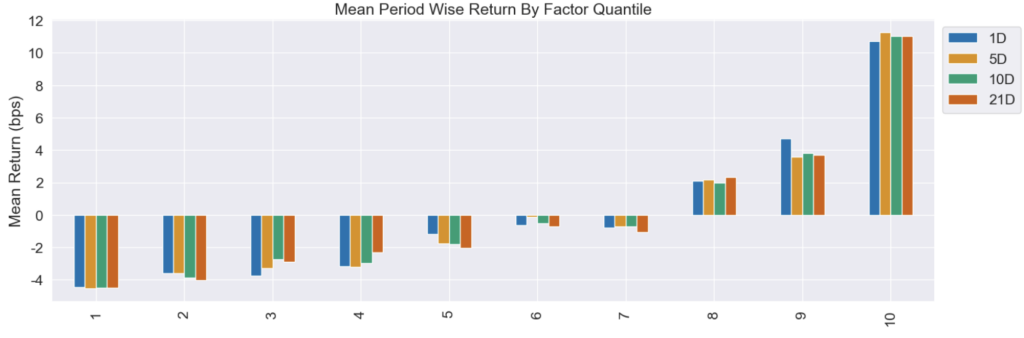
The x-axis represents the factor quantiles, where stocks are grouped into 10 categories based on their factor values. Quantile 1 represents the group with the lowest factor values, while Quantile 10 represents the group with the highest.
The y-axis represents the mean return for each quantile, measured in basis points (bps) (1 bps = 0.01%). This value indicates the average return over different holding periods (1 day, 5 days, 10 days, and 21 days).
This chart illustrates the average returns for different holding periods across various quantiles. If a factor possesses predictive power, we generally expect a monotonic relationship in the returns, where higher quantile groups (e.g., Quantile 10) yield higher average returns, while lower quantile groups (e.g., Quantile 1) yield lower returns. Such a pattern indicates that the factor can effectively construct long-short portfolios.
From the IC, IR values, and the weighted mean return of factor values, the performance of the 1-month turnover rate and 1-month price change factors did not meet the expected stability standards. Generally, a factor is considered to have strong predictive ability when its IC value is more significant than 0.03 and its IR value exceeds 0.5.
To improve the 1-month price change factor, future optimizations could be considered. Alternatively, combining these two factors with complementary factors may enhance the overall predictive ability and stability.
In the previous section, we observed that the 1-month turnover rate factor exhibited stable predictive ability and a strong monotonic trend across different holding periods, while the 1-month price change factor showed greater volatility in short-term holding periods and lacked sufficient monotonicity. This section will combine these two factors to evaluate whether the synthesized factor can effectively enhance overall predictive ability and stability.
When synthesizing multiple factors, it is essential to assign appropriate factor weights, as different factors have varying explanatory power for future returns. Proper weighting helps improve both prediction accuracy and stability.
This study uses the rank IC_IR method to calculate factor weights. The rank IC_IR is computed by dividing each factor’s one-month IR ratio by the sum of the IR ratios of both factors. This risk-adjusted IC-based weighting method assigns higher weights to factors demonstrating more extraordinary predictive ability and stability.
To simulate the signal delay effect in actual trading, we apply a lagging shift to the final weight data. Specifically, we shift the weights by one day, ensuring that only previous-period data is used, thereby avoiding the use of future information in the model.
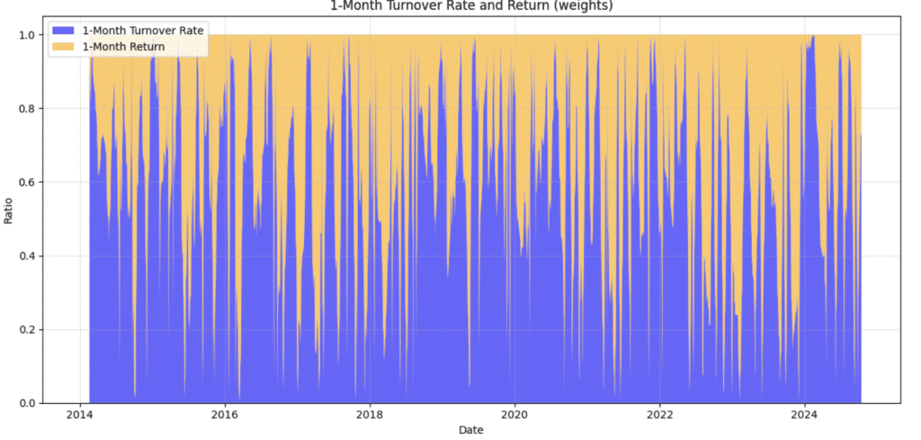
The composite factor is calculated by taking the weighted average of individual factors based on their respective weight, resulting in a single factor representing the overalleffect.
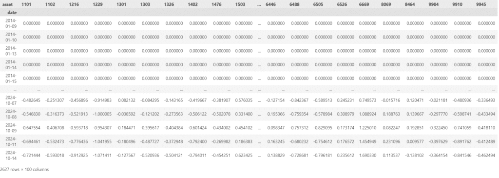
Similar to the single-factor analysis, we import the new composite factor data into Alphalens.
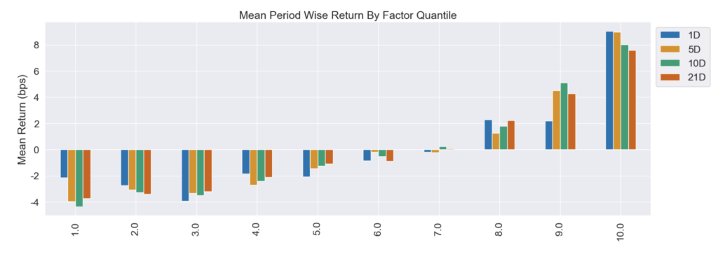
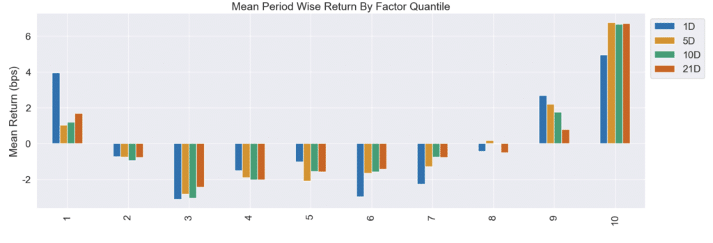
X-Axis: Represents the factor quantiles (1 to 10), where higher quantiles indicate higher factor values.
Y-Axis: Represents the mean return for each quantile, measured in basis points (bps).
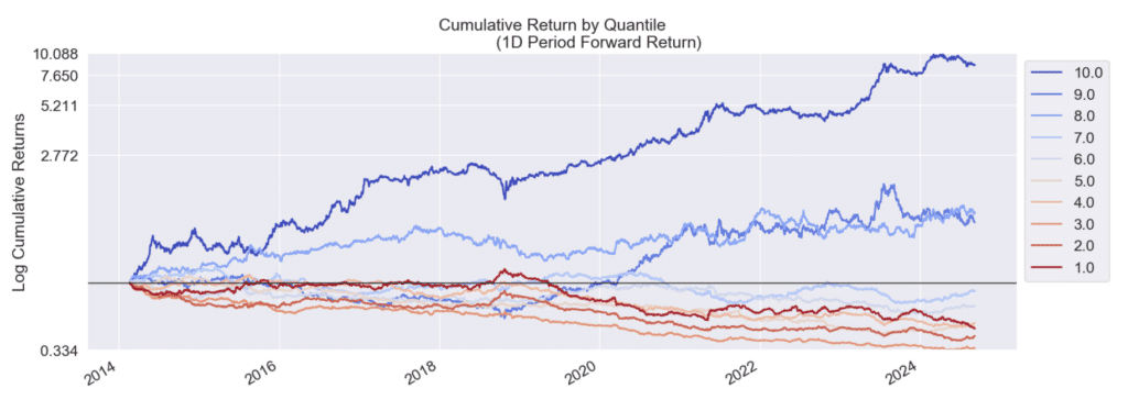
X-Axis: Represents the years, showing the time variation of cumulative returns.
Y-Axis: Represents the logarithmic cumulative return, where higher values indicate higher cumulative returns.
Color Legend: Different colored lines represent the cumulative returns of different quantiles.
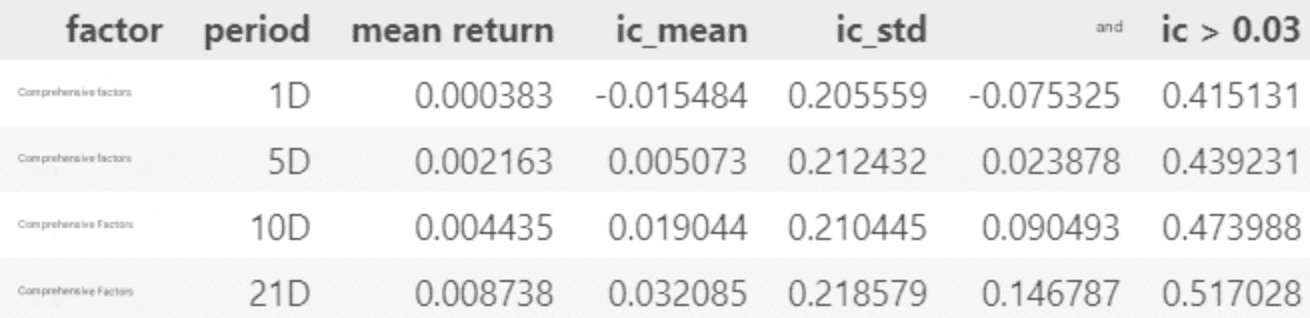
From the IC, IR values, and the weighted average return of the composite factor, we can see that the composite factor outperforms the 1-month price change factor in all holding periods in terms of IC, IR, and average return. However, it still falls slightly behind the 1-month turnover rate factor. Additionally, it is observed that the longer the holding period, the better the performance of the composite factor.
Furthermore, the bar chart of mean return by quantile shows that the composite factor exhibits a relatively stable monotonic increasing trend across quantiles, outperforming the 1-month price change factor. However, compared to the 1-month turnover rate factor, the composite factor still shows some gaps in monotonicity and stability. Overall, by integrating the characteristics of both factors, the composite factor balances predictive power and stability. However, further optimization is required to match the performance of the best-performing factor.
Through this analysis, we demonstrated how to use Alphalens to evaluate the performance of price-volume factors and apply them to practical investment strategies. The two price-volume factors analyzed in this study are the 1-month turnover rate and the 1-month price change.
From the single-factor IC and IR analysis, we found that:
We synthesized the two price-volume factors using weighted averaging. The results indicate that:
Important Reminder: This analysis is for reference only and does not constitute any product or investment advice.
We welcome readers interested in various trading strategies to consider purchasing relevant solutions from Quantitative Finance Solution. With our high-quality databases, you can construct a trading strategy that suits your needs.
“Taiwan stock market data, TEJ collect it all.”
The characteristics of the Taiwan stock market differ from those of other European and American markets. Especially in the first quarter of 2024, with the Taiwan Stock Exchange reaching a new high of 20,000 points due to the rise in TSMC’s stock price, global institutional investors are paying more attention to the performance of the Taiwan stock market.
Taiwan Economical Journal (TEJ), a financial database established in Taiwan for over 30 years, serves local financial institutions and academic institutions, and has long-term cooperation with internationally renowned data providers, providing high-quality financial data for five financial markets in Asia.
With TEJ’s assistance, you can access relevant information about major stock markets in Asia, such as securities market, financials data, enterprise operations, board of directors, sustainability data, etc., providing investors with timely and high-quality content. Additionally, TEJ offers advisory services to help solve problems in theoretical practice and financial management!
This study presents a workflow from single-factor analysis to composite factor construction and backtesting. In future applications, we can consider:
By implementing these enhancements, multi-factor strategies can become more adaptive and robust, supportinginvestment decision-making in dynamic markets.
Analyzing Factor Performance with Alphalens: Foreign Capital Factors
